import boto3
import json
import xarray as xr
import s3fs
import os
import requests
import cartopy.crs as ccrs
from matplotlib import pyplot as plt
from os import path
%matplotlib inline01. Direct cloud data access
Getting Started
In this notebook will show direct access of PO.DAAC archived products in the Earthdata Cloud in AWS Simple Storage Service (S3). In this demo, we will showcase the usage of SWOT Simulated Level-2 KaRIn SSH from GLORYS for Science Version 1. More information on the datasets can be found at https://podaac.jpl.nasa.gov/dataset/SWOT_SIMULATED_L2_KARIN_SSH_GLORYS_SCIENCE_V1.
We will access the data from inside the AWS cloud (us-west-2 region, specifically) and load a time series made of multiple netCDF files into a single xarray dataset. This approach leverages S3 native protocols for efficient access to the data.
In the future, if you want to use this notebook as a reference, please note that we are not doing collection discovery here - we assume the collection of interest has been determined.
Requirements
This can run in the Small openscapes instance, that is, it only needs 8GB of memory and ~2 CPU.
If you want to run this in your own AWS account, you can use a t2.large instance, which also has 2 CPU and 8GB memory. It’s improtant to note that all instances using direct S3 access to PO.DAAC or Earthdata data are required to run in us-west-2, or the Oregon region.
This instance will cost approximately $0.0832 per hour. The entire demo can run in considerably less time.
Imports
Most of these imports are from the Python standard library. However, you will need to install these packages into your Python 3 environment if you have not already done so:
boto3
s3fs
xarray
matplotlib
cartopy
Learning Objectives
- import needed libraries
- authenticate for NASA Earthdata archive (Earthdata Login) (here this takes place as part of obtaining the AWS credentials step)
- obtain AWS credentials for Earthdata DAAC archive in AWS S3
- access DAAC data by downloading directly into your cloud workspace from S3 within US-west 2 and operating on those files.
- access DAAC data directly from the in-region S3 bucket without moving or downloading any files to your local (cloud) workspace
- plot the first time step in the data
Note: no files are being donwloaded off the cloud, rather, we are working with the data in the AWS cloud.
Get a temporary AWS Access Key based on your Earthdata Login user ID
Direct S3 access is achieved by passing NASA supplied temporary credentials to AWS so we can interact with S3 objects (i.e. data) from applicable Earthdata Cloud buckets (storage space). For now, each NASA DAAC has different AWS credentials endpoints. Below are some of the credential endpoints to various DAACs.
The below methods (get_temp_dreds) requires the user to have a ‘netrc’ file in the users home directory.
s3_cred_endpoint = {
    'podaac':'https://archive.podaac.earthdata.nasa.gov/s3credentials',
    'gesdisc': 'https://data.gesdisc.earthdata.nasa.gov/s3credentials',
    'lpdaac':'https://data.lpdaac.earthdatacloud.nasa.gov/s3credentials',
    'ornldaac': 'https://data.ornldaac.earthdata.nasa.gov/s3credentials',
    'ghrcdaac': 'https://data.ghrc.earthdata.nasa.gov/s3credentials'
}

def get_temp_creds(provider):
    return requests.get(s3_cred_endpoint[provider]).json()
We will now get a credential for the ‘PO.DAAC’ provider and set up our environment to use those values.
NOTE if you see an error like ‘HTTP Basic: Access denied.’ It means the username/password you’ve entered is incorrect.
NOTE2 If you get what looks like a long HTML page in your error message (e.g.…), the right netrc ‘machine’ might be missing.
Location of data in the PO.DAAC S3 Archive
We need to determine the path for our products of interest. We can do this through several mechanisms. Those are described in the Finding_collection_concept_ids.ipynb notebook, or the Pre-Workshop material, https://podaac.github.io/2022-SWOT-Ocean-Cloud-Workshop/prerequisites/01_Earthdata_Search.html.
After using the Finding_collection_concept_ids.ipynb guide to find our S3 location, we end up with:
{
    ...
    "DirectDistributionInformation": {
        "Region": "us-west-2",
        "S3BucketAndObjectPrefixNames": [
            "podaac-ops-cumulus-protected/SWOT_SIMULATED_L2_KARIN_SSH_GLORYS_SCIENCE_V1/",
            "podaac-ops-cumulus-public/SWOT_SIMULATED_L2_KARIN_SSH_GLORYS_SCIENCE_V1/"
        ],
        "S3CredentialsAPIEndpoint": "https://archive.podaac.earthdata.nasa.gov/s3credentials",
        "S3CredentialsAPIDocumentationURL": "https://archive.podaac.earthdata.nasa.gov/s3credentialsREADME"
    },
    ...
}
Now that we have the S3 bucket location for the data of interest…
It’s time to find our data! Below we are using a glob to find file names matching a pattern. Here, we want any files matching the pattern used below; here this equates, in science, terms, to Cycle 001 and the first 10 passes. This information can be gleaned from product description documents. Another way of finding specific data files would be to search on cycle/pass from CMR or Earthdata Search GUI and use the S3 links provided in the resulting metadata or access links, respectively, directly instead of doing a glob (essentially an ‘ls’).
The files we are looking at are about 11-13 MB each. So the 10 we’re looking to access are about ~100 MB total.
['podaac-ops-cumulus-protected/SWOT_SIMULATED_L2_KARIN_SSH_GLORYS_SCIENCE_V1/SWOT_L2_LR_SSH_Expert_001_001_20140412T120000_20140412T125126_DG10_01.nc',
 'podaac-ops-cumulus-protected/SWOT_SIMULATED_L2_KARIN_SSH_GLORYS_SCIENCE_V1/SWOT_L2_LR_SSH_Expert_001_002_20140412T125126_20140412T134253_DG10_01.nc',
 'podaac-ops-cumulus-protected/SWOT_SIMULATED_L2_KARIN_SSH_GLORYS_SCIENCE_V1/SWOT_L2_LR_SSH_Expert_001_003_20140412T134253_20140412T143420_DG10_01.nc',
 'podaac-ops-cumulus-protected/SWOT_SIMULATED_L2_KARIN_SSH_GLORYS_SCIENCE_V1/SWOT_L2_LR_SSH_Expert_001_004_20140412T143420_20140412T152546_DG10_01.nc',
 'podaac-ops-cumulus-protected/SWOT_SIMULATED_L2_KARIN_SSH_GLORYS_SCIENCE_V1/SWOT_L2_LR_SSH_Expert_001_005_20140412T152547_20140412T161713_DG10_01.nc',
 'podaac-ops-cumulus-protected/SWOT_SIMULATED_L2_KARIN_SSH_GLORYS_SCIENCE_V1/SWOT_L2_LR_SSH_Expert_001_006_20140412T161714_20140412T170840_DG10_01.nc',
 'podaac-ops-cumulus-protected/SWOT_SIMULATED_L2_KARIN_SSH_GLORYS_SCIENCE_V1/SWOT_L2_LR_SSH_Expert_001_007_20140412T170840_20140412T180007_DG10_01.nc',
 'podaac-ops-cumulus-protected/SWOT_SIMULATED_L2_KARIN_SSH_GLORYS_SCIENCE_V1/SWOT_L2_LR_SSH_Expert_001_008_20140412T180008_20140412T185134_DG10_01.nc',
 'podaac-ops-cumulus-protected/SWOT_SIMULATED_L2_KARIN_SSH_GLORYS_SCIENCE_V1/SWOT_L2_LR_SSH_Expert_001_009_20140412T185134_20140412T194301_DG10_01.nc']
Traditional Access: get files from S3 and store them on your running cloud instance
Here we will leverage the speed of transfering data within the cloud to our running instance (this notebook!). We will download 10 files into the ‘DEMO_FILES’ directory to show you cloud and traditional access.
CPU times: user 335 ms, sys: 255 ms, total: 590 ms
Wall time: 5.34 sCPU times: user 1.25 s, sys: 38.7 ms, total: 1.29 s
Wall time: 2.15 s<xarray.Dataset>
Dimensions: (num_lines: 88796, num_pixels: 71,
num_sides: 2)
Coordinates:
latitude (num_lines, num_pixels) float64 dask.array<chunksize=(9866, 71), meta=np.ndarray>
longitude (num_lines, num_pixels) float64 dask.array<chunksize=(9866, 71), meta=np.ndarray>
latitude_nadir (num_lines) float64 dask.array<chunksize=(9866,), meta=np.ndarray>
longitude_nadir (num_lines) float64 dask.array<chunksize=(9866,), meta=np.ndarray>
Dimensions without coordinates: num_lines, num_pixels, num_sides
Data variables: (12/91)
time (num_lines) float64 dask.array<chunksize=(9866,), meta=np.ndarray>
time_tai (num_lines) float64 dask.array<chunksize=(9866,), meta=np.ndarray>
ssh_karin (num_lines, num_pixels) float64 dask.array<chunksize=(9866, 71), meta=np.ndarray>
ssh_karin_uncert (num_lines, num_pixels) float32 dask.array<chunksize=(9866, 71), meta=np.ndarray>
ssha_karin (num_lines, num_pixels) float64 dask.array<chunksize=(9866, 71), meta=np.ndarray>
ssh_karin_2 (num_lines, num_pixels) float64 dask.array<chunksize=(9866, 71), meta=np.ndarray>
... ...
simulated_error_baseline_dilation (num_lines, num_pixels) float64 dask.array<chunksize=(9866, 71), meta=np.ndarray>
simulated_error_timing (num_lines, num_pixels) float64 dask.array<chunksize=(9866, 71), meta=np.ndarray>
simulated_error_roll (num_lines, num_pixels) float64 dask.array<chunksize=(9866, 71), meta=np.ndarray>
simulated_error_phase (num_lines, num_pixels) float64 dask.array<chunksize=(9866, 71), meta=np.ndarray>
simulated_error_orbital (num_lines, num_pixels) float64 dask.array<chunksize=(9866, 71), meta=np.ndarray>
simulated_error_karin (num_lines, num_pixels) float64 dask.array<chunksize=(9866, 71), meta=np.ndarray>
Attributes: (12/32)
Conventions: CF-1.7
title: Level 2 Low Rate Sea Surface Height Data Prod...
institution: CNES/JPL
source: Simulate product
history: 2021-09-10 09:54:55Z : Creation
platform: SWOT
... ...
right_last_longitude: 131.81928697472432
right_last_latitude: 77.03254381435897
wavelength: 0.008385803020979
orbit_solution: POE
ellipsoid_semi_major_axis: 6378137.0
ellipsoid_flattening: 0.003352810664781205xarray.Dataset
- num_lines: 88796
- num_pixels: 71
- num_sides: 2
- latitude(num_lines, num_pixels)float64dask.array<chunksize=(9866, 71), meta=np.ndarray>
- long_name :
- latitude (positive N, negative S)
- standard_name :
- latitude
- units :
- degrees_north
- valid_min :
- -80000000
- valid_max :
- 80000000
- comment :
- Latitude of measurement [-80,80]. Positive latitude is North latitude, negative latitude is South latitude.
Array Chunk Bytes 48.10 MiB 5.35 MiB Shape (88796, 71) (9869, 71) Count 27 Tasks 9 Chunks Type float64 numpy.ndarray - longitude(num_lines, num_pixels)float64dask.array<chunksize=(9866, 71), meta=np.ndarray>
- long_name :
- longitude (degrees East)
- standard_name :
- longitude
- units :
- degrees_east
- valid_min :
- 0
- valid_max :
- 359999999
- comment :
- Longitude of measurement. East longitude relative to Greenwich meridian.
Array Chunk Bytes 48.10 MiB 5.35 MiB Shape (88796, 71) (9869, 71) Count 27 Tasks 9 Chunks Type float64 numpy.ndarray - latitude_nadir(num_lines)float64dask.array<chunksize=(9866,), meta=np.ndarray>
- long_name :
- latitude of satellite nadir point
- standard_name :
- latitude
- units :
- degrees_north
- valid_min :
- -80000000
- valid_max :
- 80000000
- comment :
- Geodetic latitude [-80,80] (degrees north of equator) of the satellite nadir point.
Array Chunk Bytes 693.72 kiB 77.10 kiB Shape (88796,) (9869,) Count 27 Tasks 9 Chunks Type float64 numpy.ndarray - longitude_nadir(num_lines)float64dask.array<chunksize=(9866,), meta=np.ndarray>
- long_name :
- longitude of satellite nadir point
- standard_name :
- longitude
- units :
- degrees_east
- valid_min :
- 0
- valid_max :
- 359999999
- comment :
- Longitude (degrees east of Grenwich meridian) of the satellite nadir point.
Array Chunk Bytes 693.72 kiB 77.10 kiB Shape (88796,) (9869,) Count 27 Tasks 9 Chunks Type float64 numpy.ndarray
- time(num_lines)float64dask.array<chunksize=(9866,), meta=np.ndarray>
- long_name :
- time in UTC
- standard_name :
- time
- calendar :
- gregorian
- leap_second :
- YYYY-MM-DDThh:mm:ssZ
- units :
- seconds since 2000-01-01 00:00:00.0
- comment :
- Time of measurement in seconds in the UTC time scale since 1 Jan 2000 00:00:00 UTC. [tai_utc_difference] is the difference between TAI and UTC reference time (seconds) for the first measurement of the data set. If a leap second occurs within the data set, the attribute leap_second is set to the UTC time at which the leap second occurs.
- tai_utc_difference :
- 35.0
Array Chunk Bytes 693.72 kiB 77.10 kiB Shape (88796,) (9869,) Count 27 Tasks 9 Chunks Type float64 numpy.ndarray - time_tai(num_lines)float64dask.array<chunksize=(9866,), meta=np.ndarray>
- long_name :
- time in TAI
- standard_name :
- time
- calendar :
- gregorian
- tai_utc_difference :
- [Value of TAI-UTC at time of first record]
- units :
- seconds since 2000-01-01 00:00:00.0
- comment :
- Time of measurement in seconds in the TAI time scale since 1 Jan 2000 00:00:00 TAI. This time scale contains no leap seconds. The difference (in seconds) with time in UTC is given by the attribute [time:tai_utc_difference].
Array Chunk Bytes 693.72 kiB 77.10 kiB Shape (88796,) (9869,) Count 27 Tasks 9 Chunks Type float64 numpy.ndarray - ssh_karin(num_lines, num_pixels)float64dask.array<chunksize=(9866, 71), meta=np.ndarray>
- long_name :
- sea surface height
- standard_name :
- sea surface height above reference ellipsoid
- units :
- m
- valid_min :
- -15000000
- valid_max :
- 150000000
- comment :
- Fully corrected sea surface height measured by KaRIn. The height is relative to the reference ellipsoid defined in the global attributes. This value is computed using radiometer measurements for wet troposphere effects on the KaRIn measurement (e.g., rad_wet_tropo_cor and sea_state_bias_cor).
Array Chunk Bytes 48.10 MiB 5.35 MiB Shape (88796, 71) (9869, 71) Count 27 Tasks 9 Chunks Type float64 numpy.ndarray - ssh_karin_uncert(num_lines, num_pixels)float32dask.array<chunksize=(9866, 71), meta=np.ndarray>
- long_name :
- sea surface height anomaly uncertainty
- units :
- m
- valid_min :
- 0
- valid_max :
- 60000
- comment :
- 1-sigma uncertainty on the sea surface height from the KaRIn measurement.
Array Chunk Bytes 24.05 MiB 2.67 MiB Shape (88796, 71) (9869, 71) Count 27 Tasks 9 Chunks Type float32 numpy.ndarray - ssha_karin(num_lines, num_pixels)float64dask.array<chunksize=(9866, 71), meta=np.ndarray>
- long_name :
- sea surface height anomaly
- units :
- m
- valid_min :
- -1000000
- valid_max :
- 1000000
- comment :
- Sea surface height anomaly from the KaRIn measurement = ssh_karin - mean_sea_surface_cnescls - solid_earth_tide - ocean_tide_fes – internal_tide_hret - pole_tide - dac.
Array Chunk Bytes 48.10 MiB 5.35 MiB Shape (88796, 71) (9869, 71) Count 27 Tasks 9 Chunks Type float64 numpy.ndarray - ssh_karin_2(num_lines, num_pixels)float64dask.array<chunksize=(9866, 71), meta=np.ndarray>
- long_name :
- sea surface height
- standard_name :
- sea surface height above reference ellipsoid
- units :
- m
- valid_min :
- -15000000
- valid_max :
- 150000000
- comment :
- Fully corrected sea surface height measured by KaRIn. The height is relative to the reference ellipsoid defined in the global attributes. This value is computed using model-based estimates for wet troposphere effects on the KaRIn measurement (e.g., model_wet_tropo_cor and sea_state_bias_cor_2).
Array Chunk Bytes 48.10 MiB 5.35 MiB Shape (88796, 71) (9869, 71) Count 27 Tasks 9 Chunks Type float64 numpy.ndarray - ssha_karin_2(num_lines, num_pixels)float64dask.array<chunksize=(9866, 71), meta=np.ndarray>
- long_name :
- sea surface height anomaly
- units :
- m
- valid_min :
- -1000000
- valid_max :
- 1000000
- comment :
- Sea surface height anomaly from the KaRIn measurement = ssh_karin_2 - mean_sea_surface_cnescls - solid_earth_tide - ocean_tide_fes – internal_tide_hret - pole_tide - dac.
Array Chunk Bytes 48.10 MiB 5.35 MiB Shape (88796, 71) (9869, 71) Count 27 Tasks 9 Chunks Type float64 numpy.ndarray - ssha_karin_qual(num_lines, num_pixels)float64dask.array<chunksize=(9866, 71), meta=np.ndarray>
- long_name :
- sea surface height quality flag
- standard_name :
- status_flag
- flag_meanings :
- good bad
- flag_values :
- [0 1]
- valid_min :
- 0
- valid_max :
- 1
- comment :
- Quality flag for the SSHA from KaRIn.
Array Chunk Bytes 48.10 MiB 5.35 MiB Shape (88796, 71) (9869, 71) Count 27 Tasks 9 Chunks Type float64 numpy.ndarray - polarization_karin(num_lines, num_sides)objectdask.array<chunksize=(9866, 2), meta=np.ndarray>
- long_name :
- polarization for each side of the KaRIn swath
- comment :
- H denotes co-polarized linear horizontal, V denotes co-polarized linear vertical.
Array Chunk Bytes 1.35 MiB 154.20 kiB Shape (88796, 2) (9869, 2) Count 27 Tasks 9 Chunks Type object numpy.ndarray - swh_karin(num_lines, num_pixels)float32dask.array<chunksize=(9866, 71), meta=np.ndarray>
- long_name :
- significant wave height from KaRIn
- standard_name :
- sea_surface_wave_significant_height
- units :
- m
- valid_min :
- 0
- valid_max :
- 25000
- comment :
- Significant wave height from KaRIn volumetric correlation.
Array Chunk Bytes 24.05 MiB 2.67 MiB Shape (88796, 71) (9869, 71) Count 27 Tasks 9 Chunks Type float32 numpy.ndarray - swh_karin_uncert(num_lines, num_pixels)float32dask.array<chunksize=(9866, 71), meta=np.ndarray>
- long_name :
- 1-sigma uncertainty on significant wave height from KaRIn
- units :
- m
- valid_min :
- 0
- valid_max :
- 25000
- comment :
- 1-sigma uncertainty on significant wave height from KaRIn.
Array Chunk Bytes 24.05 MiB 2.67 MiB Shape (88796, 71) (9869, 71) Count 27 Tasks 9 Chunks Type float32 numpy.ndarray - sig0_karin(num_lines, num_pixels)float32dask.array<chunksize=(9866, 71), meta=np.ndarray>
- long_name :
- normalized radar cross section (sigma0) from KaRIn
- standard_name :
- surface_backwards_scattering_coefficient_of_radar_wave
- units :
- 1
- valid_min :
- -1000.0
- valid_max :
- 10000000.0
- comment :
- Normalized radar cross section (sigma0) from KaRIn in real, linear units (not decibels). The value may be negative due to noise subtraction. The value is corrected for instrument calibration and atmospheric attenuation. Radiometer measurements provide the atmospheric attenuation (sig0_cor_atmos_rad).
Array Chunk Bytes 24.05 MiB 2.67 MiB Shape (88796, 71) (9869, 71) Count 27 Tasks 9 Chunks Type float32 numpy.ndarray - sig0_karin_uncert(num_lines, num_pixels)float32dask.array<chunksize=(9866, 71), meta=np.ndarray>
- long_name :
- 1-sigma uncertainty on sigma0 from KaRIn
- units :
- 1
- valid_min :
- 0.0
- valid_max :
- 1000.0
- comment :
- 1-sigma uncertainty on sigma0 from KaRIn.
Array Chunk Bytes 24.05 MiB 2.67 MiB Shape (88796, 71) (9869, 71) Count 27 Tasks 9 Chunks Type float32 numpy.ndarray - sig0_karin_2(num_lines, num_pixels)float32dask.array<chunksize=(9866, 71), meta=np.ndarray>
- long_name :
- normalized radar cross section (sigma0) from KaRIn
- standard_name :
- surface_backwards_scattering_coefficient_of_radar_wave
- units :
- 1
- valid_min :
- -1000.0
- valid_max :
- 10000000.0
- comment :
- Normalized radar cross section (sigma0) from KaRIn in real, linear units (not decibels). The value may be negative due to noise subtraction. The value is corrected for instrument calibration and atmospheric attenuation. A meteorological model provides the atmospheric attenuation (sig0_cor_atmos_model).
Array Chunk Bytes 24.05 MiB 2.67 MiB Shape (88796, 71) (9869, 71) Count 27 Tasks 9 Chunks Type float32 numpy.ndarray - wind_speed_karin(num_lines, num_pixels)float32dask.array<chunksize=(9866, 71), meta=np.ndarray>
- long_name :
- wind speed from KaRIn
- standard_name :
- wind_speed
- source :
- TBD
- units :
- m/s
- valid_min :
- 0
- valid_max :
- 65000
- comment :
- Wind speed from KaRIn computed from sig0_karin.
Array Chunk Bytes 24.05 MiB 2.67 MiB Shape (88796, 71) (9869, 71) Count 27 Tasks 9 Chunks Type float32 numpy.ndarray - wind_speed_karin_2(num_lines, num_pixels)float32dask.array<chunksize=(9866, 71), meta=np.ndarray>
- long_name :
- wind speed from KaRIn
- standard_name :
- wind_speed
- source :
- TBD
- units :
- m/s
- valid_min :
- 0
- valid_max :
- 65000
- comment :
- Wind speed from KaRIn computed from sig0_karin_2.
Array Chunk Bytes 24.05 MiB 2.67 MiB Shape (88796, 71) (9869, 71) Count 27 Tasks 9 Chunks Type float32 numpy.ndarray - swh_karin_qual(num_lines, num_pixels)float64dask.array<chunksize=(9866, 71), meta=np.ndarray>
- long_name :
- quality flag for significant wave height from KaRIn.
- standard_name :
- status_flag
- flag_meanings :
- good bad
- flag_values :
- [0 1]
- valid_min :
- 0
- valid_max :
- 1
- comment :
- Quality flag for significant wave height from KaRIn.
Array Chunk Bytes 48.10 MiB 5.35 MiB Shape (88796, 71) (9869, 71) Count 27 Tasks 9 Chunks Type float64 numpy.ndarray - sig0_karin_qual(num_lines, num_pixels)float64dask.array<chunksize=(9866, 71), meta=np.ndarray>
- long_name :
- quality flag for sigma0 from KaRIn.
- standard_name :
- status_flag
- flag_meanings :
- good bad
- flag_values :
- [0 1]
- valid_min :
- 0
- valid_max :
- 1
- comment :
- Quality flag for sigma0 from KaRIn.
Array Chunk Bytes 48.10 MiB 5.35 MiB Shape (88796, 71) (9869, 71) Count 27 Tasks 9 Chunks Type float64 numpy.ndarray - num_pt_avg(num_lines, num_pixels)float32dask.array<chunksize=(9866, 71), meta=np.ndarray>
- long_name :
- number of samples averaged
- units :
- 1
- valid_min :
- 0
- valid_max :
- 289
- comment :
- Number of native unsmoothed, beam-combined KaRIn samples averaged.
Array Chunk Bytes 24.05 MiB 2.67 MiB Shape (88796, 71) (9869, 71) Count 27 Tasks 9 Chunks Type float32 numpy.ndarray - swh_model(num_lines, num_pixels)float32dask.array<chunksize=(9866, 71), meta=np.ndarray>
- long_name :
- significant wave height from wave model
- standard_name :
- sea_surface_wave_significant_height
- source :
- European Centre for Medium-Range Weather Forecasts
- institution :
- ECMWF
- units :
- m
- valid_min :
- 0
- valid_max :
- 30000
- comment :
- Significant wave height from model.
Array Chunk Bytes 24.05 MiB 2.67 MiB Shape (88796, 71) (9869, 71) Count 27 Tasks 9 Chunks Type float32 numpy.ndarray - mean_wave_direction(num_lines, num_pixels)float32dask.array<chunksize=(9866, 71), meta=np.ndarray>
- long_name :
- mean sea surface wave direction
- source :
- Meteo France Wave Model (MF-WAM)
- institution :
- Meteo France
- units :
- degree
- valid_min :
- 0
- valid_max :
- 36000
- comment :
- Mean sea surface wave direction.
Array Chunk Bytes 24.05 MiB 2.67 MiB Shape (88796, 71) (9869, 71) Count 27 Tasks 9 Chunks Type float32 numpy.ndarray - mean_wave_period_t02(num_lines, num_pixels)float32dask.array<chunksize=(9866, 71), meta=np.ndarray>
- long_name :
- sea surface wind wave mean period
- standard_name :
- sea_surface_wave_significant_period
- source :
- Meteo France Wave Model (MF-WAM)
- institution :
- Meteo France
- units :
- s
- valid_min :
- 0
- valid_max :
- 100
- comment :
- Sea surface wind wave mean period from model spectral density second moment.
Array Chunk Bytes 24.05 MiB 2.67 MiB Shape (88796, 71) (9869, 71) Count 27 Tasks 9 Chunks Type float32 numpy.ndarray - wind_speed_model_u(num_lines, num_pixels)float32dask.array<chunksize=(9866, 71), meta=np.ndarray>
- long_name :
- u component of model wind
- standard_name :
- eastward_wind
- source :
- European Centre for Medium-Range Weather Forecasts
- institution :
- ECMWF
- units :
- m/s
- valid_min :
- -30000
- valid_max :
- 30000
- comment :
- Eastward component of the atmospheric model wind vector at 10 meters.
Array Chunk Bytes 24.05 MiB 2.67 MiB Shape (88796, 71) (9869, 71) Count 27 Tasks 9 Chunks Type float32 numpy.ndarray - wind_speed_model_v(num_lines, num_pixels)float32dask.array<chunksize=(9866, 71), meta=np.ndarray>
- long_name :
- v component of model wind
- standard_name :
- northward_wind
- source :
- European Centre for Medium-Range Weather Forecasts
- institution :
- ECMWF
- units :
- m/s
- valid_min :
- -30000
- valid_max :
- 30000
- comment :
- Northward component of the atmospheric model wind vector at 10 meters.
Array Chunk Bytes 24.05 MiB 2.67 MiB Shape (88796, 71) (9869, 71) Count 27 Tasks 9 Chunks Type float32 numpy.ndarray - wind_speed_rad(num_lines, num_sides)float32dask.array<chunksize=(9866, 2), meta=np.ndarray>
- long_name :
- wind speed from radiometer
- standard_name :
- wind_speed
- source :
- Advanced Microwave Radiometer
- units :
- m/s
- valid_min :
- 0
- valid_max :
- 65000
- comment :
- Wind speed from radiometer measurements.
Array Chunk Bytes 693.72 kiB 77.10 kiB Shape (88796, 2) (9869, 2) Count 27 Tasks 9 Chunks Type float32 numpy.ndarray - distance_to_coast(num_lines, num_pixels)float32dask.array<chunksize=(9866, 71), meta=np.ndarray>
- long_name :
- distance to coast
- source :
- MODIS/GlobCover
- institution :
- European Space Agency
- units :
- m
- valid_min :
- 0
- valid_max :
- 21000
- comment :
- Approximate distance to the nearest coast point along the Earth surface.
Array Chunk Bytes 24.05 MiB 2.67 MiB Shape (88796, 71) (9869, 71) Count 27 Tasks 9 Chunks Type float32 numpy.ndarray - heading_to_coast(num_lines, num_pixels)float32dask.array<chunksize=(9866, 71), meta=np.ndarray>
- long_name :
- heading to coast
- units :
- degrees
- valid_min :
- 0
- valid_max :
- 35999
- comment :
- Approximate compass heading (0-360 degrees with respect to true north) to the nearest coast point.
Array Chunk Bytes 24.05 MiB 2.67 MiB Shape (88796, 71) (9869, 71) Count 27 Tasks 9 Chunks Type float32 numpy.ndarray - ancillary_surface_classification_flag(num_lines, num_pixels)float32dask.array<chunksize=(9866, 71), meta=np.ndarray>
- long_name :
- surface classification
- standard_name :
- status_flag
- source :
- MODIS/GlobCover
- institution :
- European Space Agency
- flag_meanings :
- open_ocean land continental_water aquatic_vegetation continental_ice_snow floating_ice salted_basin
- flag_values :
- [0 1 2 3 4 5 6]
- valid_min :
- 0
- valid_max :
- 6
- comment :
- 7-state surface type classification computed from a mask built with MODIS and GlobCover data.
Array Chunk Bytes 24.05 MiB 2.67 MiB Shape (88796, 71) (9869, 71) Count 27 Tasks 9 Chunks Type float32 numpy.ndarray - dynamic_ice_flag(num_lines, num_pixels)float32dask.array<chunksize=(9866, 71), meta=np.ndarray>
- long_name :
- dynamic ice flag
- standard_name :
- status_flag
- source :
- EUMETSAT Ocean and Sea Ice Satellite Applications Facility
- institution :
- EUMETSAT
- flag_meanings :
- no_ice probable_ice ice
- flag_values :
- [0 1 2]
- valid_min :
- 0
- valid_max :
- 2
- comment :
- Dynamic ice flag for the location of the KaRIn measurement.
Array Chunk Bytes 24.05 MiB 2.67 MiB Shape (88796, 71) (9869, 71) Count 27 Tasks 9 Chunks Type float32 numpy.ndarray - rain_flag(num_lines, num_pixels)float32dask.array<chunksize=(9866, 71), meta=np.ndarray>
- long_name :
- rain flag
- standard_name :
- status_flag
- flag_meanings :
- no_rain probable_rain rain
- flag_values :
- [0 1 2]
- valid_min :
- 0
- valid_max :
- 2
- comment :
- Flag indicates that signal is attenuated, probably from rain.
Array Chunk Bytes 24.05 MiB 2.67 MiB Shape (88796, 71) (9869, 71) Count 27 Tasks 9 Chunks Type float32 numpy.ndarray - rad_surface_type_flag(num_lines, num_sides)float32dask.array<chunksize=(9866, 2), meta=np.ndarray>
- long_name :
- radiometer surface type flag
- standard_name :
- status_flag
- source :
- Advanced Microwave Radiometer
- flag_meanings :
- open_ocean coastal_ocean land
- flag_values :
- [0 1 2]
- valid_min :
- 0
- valid_max :
- 2
- comment :
- Flag indicating the validity and type of processing applied to generate the wet troposphere correction (rad_wet_tropo_cor). A value of 0 indicates that open ocean processing is used, a value of 1 indicates coastal processing, and a value of 2 indicates that rad_wet_tropo_cor is invalid due to land contamination.
Array Chunk Bytes 693.72 kiB 77.10 kiB Shape (88796, 2) (9869, 2) Count 27 Tasks 9 Chunks Type float32 numpy.ndarray - sc_altitude(num_lines)float64dask.array<chunksize=(9866,), meta=np.ndarray>
- long_name :
- altitude of KMSF origin
- standard_name :
- height_above_reference_ellipsoid
- units :
- m
- valid_min :
- 0
- valid_max :
- 2000000000
- comment :
- Altitude of the KMSF origin.
Array Chunk Bytes 693.72 kiB 77.10 kiB Shape (88796,) (9869,) Count 27 Tasks 9 Chunks Type float64 numpy.ndarray - orbit_alt_rate(num_lines)float32dask.array<chunksize=(9866,), meta=np.ndarray>
- long_name :
- orbital altitude rate with respect to mean sea surface
- units :
- m/s
- valid_min :
- -3500
- valid_max :
- 3500
- comment :
- Orbital altitude rate with respect to the mean sea surface.
Array Chunk Bytes 346.86 kiB 38.55 kiB Shape (88796,) (9869,) Count 27 Tasks 9 Chunks Type float32 numpy.ndarray - cross_track_angle(num_lines)float64dask.array<chunksize=(9866,), meta=np.ndarray>
- long_name :
- cross-track angle from true north
- units :
- degrees
- valid_min :
- 0
- valid_max :
- 359999999
- comment :
- Angle with respect to true north of the cross-track direction to the right of the spacecraft velocity vector.
Array Chunk Bytes 693.72 kiB 77.10 kiB Shape (88796,) (9869,) Count 27 Tasks 9 Chunks Type float64 numpy.ndarray - sc_roll(num_lines)float64dask.array<chunksize=(9866,), meta=np.ndarray>
- long_name :
- roll of the spacecraft
- standard_name :
- platform_roll_angle
- units :
- degrees
- valid_min :
- -1799999
- valid_max :
- 1800000
- comment :
- KMSF attitude roll angle; positive values move the +y antenna down.
Array Chunk Bytes 693.72 kiB 77.10 kiB Shape (88796,) (9869,) Count 27 Tasks 9 Chunks Type float64 numpy.ndarray - sc_pitch(num_lines)float64dask.array<chunksize=(9866,), meta=np.ndarray>
- long_name :
- pitch of the spacecraft
- standard_name :
- platform_pitch_angle
- units :
- degrees
- valid_min :
- -1799999
- valid_max :
- 1800000
- comment :
- KMSF attitude pitch angle; positive values move the KMSF +x axis up.
Array Chunk Bytes 693.72 kiB 77.10 kiB Shape (88796,) (9869,) Count 27 Tasks 9 Chunks Type float64 numpy.ndarray - sc_yaw(num_lines)float64dask.array<chunksize=(9866,), meta=np.ndarray>
- long_name :
- yaw of the spacecraft
- standard_name :
- platform_yaw_angle
- units :
- degrees
- valid_min :
- -1799999
- valid_max :
- 1800000
- comment :
- KMSF attitude yaw angle relative to the nadir track. The yaw angle is a right-handed rotation about the nadir (downward) direction. A yaw value of 0 deg indicates that the KMSF +x axis is aligned with the horizontal component of the Earth-relative velocity vector. A yaw value of 180 deg indicates that the spacecraft is in a yaw-flipped state, with the KMSF -x axis aligned with the horizontal component of the Earth-relative velocity vector.
Array Chunk Bytes 693.72 kiB 77.10 kiB Shape (88796,) (9869,) Count 27 Tasks 9 Chunks Type float64 numpy.ndarray - velocity_heading(num_lines)float64dask.array<chunksize=(9866,), meta=np.ndarray>
- long_name :
- heading of the spacecraft Earth-relative velocity vector
- units :
- degrees
- valid_min :
- 0
- valid_max :
- 359999999
- comment :
- Angle with respect to true north of the horizontal component of the spacecraft Earth-relative velocity vector. A value of 90 deg indicates that the spacecraft velocity vector pointed due east. Values between 0 and 90 deg indicate that the velocity vector has a northward component, and values between 90 and 180 deg indicate that the velocity vector has a southward component.
Array Chunk Bytes 693.72 kiB 77.10 kiB Shape (88796,) (9869,) Count 27 Tasks 9 Chunks Type float64 numpy.ndarray - orbit_qual(num_lines)float32dask.array<chunksize=(9866,), meta=np.ndarray>
- long_name :
- orbit quality flag
- standard_name :
- status_flag
- valid_min :
- 0
- valid_max :
- 1
- comment :
- Orbit quality flag.
Array Chunk Bytes 346.86 kiB 38.55 kiB Shape (88796,) (9869,) Count 27 Tasks 9 Chunks Type float32 numpy.ndarray - latitude_avg_ssh(num_lines, num_pixels)float64dask.array<chunksize=(9866, 71), meta=np.ndarray>
- long_name :
- weighted average latitude of samples used to compute SSH
- standard_name :
- latitude
- units :
- degrees_north
- valid_min :
- -80000000
- valid_max :
- 80000000
- comment :
- Latitude of measurement [-80,80]. Positive latitude is North latitude, negative latitude is South latitude. This value may be biased away from a nominal grid location if some of the native, unsmoothed samples were discarded during processing.
Array Chunk Bytes 48.10 MiB 5.35 MiB Shape (88796, 71) (9869, 71) Count 27 Tasks 9 Chunks Type float64 numpy.ndarray - longitude_avg_ssh(num_lines, num_pixels)float64dask.array<chunksize=(9866, 71), meta=np.ndarray>
- long_name :
- weighted average longitude of samples used to compute SSH
- standard_name :
- longitude
- units :
- degrees_east
- valid_min :
- 0
- valid_max :
- 359999999
- comment :
- Longitude of measurement. East longitude relative to Greenwich meridian. This value may be biased away from a nominal grid location if some of the native, unsmoothed samples were discarded during processing.
Array Chunk Bytes 48.10 MiB 5.35 MiB Shape (88796, 71) (9869, 71) Count 27 Tasks 9 Chunks Type float64 numpy.ndarray - cross_track_distance(num_lines, num_pixels)float32dask.array<chunksize=(9866, 71), meta=np.ndarray>
- long_name :
- cross track distance
- units :
- m
- valid_min :
- -75000.0
- valid_max :
- 75000.0
- comment :
- Distance of sample from nadir. Negative values indicate the left side of the swath, and positive values indicate the right side of the swath.
Array Chunk Bytes 24.05 MiB 2.67 MiB Shape (88796, 71) (9869, 71) Count 27 Tasks 9 Chunks Type float32 numpy.ndarray - x_factor(num_lines, num_pixels)float32dask.array<chunksize=(9866, 71), meta=np.ndarray>
- long_name :
- radiometric calibration X factor as a composite value for the X factors of the +y and -y channels
- units :
- 1
- valid_min :
- 0.0
- valid_max :
- 1e+20
- comment :
- Radiometric calibration X factor as a linear power ratio.
Array Chunk Bytes 24.05 MiB 2.67 MiB Shape (88796, 71) (9869, 71) Count 27 Tasks 9 Chunks Type float32 numpy.ndarray - sig0_cor_atmos_model(num_lines, num_pixels)float32dask.array<chunksize=(9866, 71), meta=np.ndarray>
- long_name :
- two-way atmospheric correction to sigma0 from model
- source :
- European Centre for Medium-Range Weather Forecasts
- institution :
- ECMWF
- units :
- 1
- valid_min :
- 1.0
- valid_max :
- 10.0
- comment :
- Atmospheric correction to sigma0 from weather model data as a linear power multiplier (not decibels). sig0_cor_atmos_model is already applied in computing sig0_karin_2.
Array Chunk Bytes 24.05 MiB 2.67 MiB Shape (88796, 71) (9869, 71) Count 27 Tasks 9 Chunks Type float32 numpy.ndarray - sig0_cor_atmos_rad(num_lines, num_pixels)float32dask.array<chunksize=(9866, 71), meta=np.ndarray>
- long_name :
- two-way atmospheric correction to sigma0 from radiometer data
- source :
- Advanced Microwave Radiometer
- units :
- 1
- valid_min :
- 1.0
- valid_max :
- 10.0
- comment :
- Atmospheric correction to sigma0 from radiometer data as a linear power multiplier (not decibels). sig0_cor_atmos_rad is already applied in computing sig0_karin.
Array Chunk Bytes 24.05 MiB 2.67 MiB Shape (88796, 71) (9869, 71) Count 27 Tasks 9 Chunks Type float32 numpy.ndarray - doppler_centroid(num_lines, num_sides)float32dask.array<chunksize=(9866, 2), meta=np.ndarray>
- long_name :
- doppler centroid estimated by KaRIn
- units :
- 1/s
- valid_min :
- -30000
- valid_max :
- 30000
- comment :
- Doppler centroid (in hertz or cycles per second) estimated by KaRIn.
Array Chunk Bytes 693.72 kiB 77.10 kiB Shape (88796, 2) (9869, 2) Count 27 Tasks 9 Chunks Type float32 numpy.ndarray - phase_bias_ref_surface(num_lines, num_pixels)float64dask.array<chunksize=(9866, 71), meta=np.ndarray>
- long_name :
- height of reference surface used for phase bias calculation
- units :
- m
- valid_min :
- -15000000
- valid_max :
- 150000000
- comment :
- Height (relative to the reference ellipsoid) of the reference surface used for phase bias calculation during L1B processing.
Array Chunk Bytes 48.10 MiB 5.35 MiB Shape (88796, 71) (9869, 71) Count 27 Tasks 9 Chunks Type float64 numpy.ndarray - obp_ref_surface(num_lines, num_pixels)float64dask.array<chunksize=(9866, 71), meta=np.ndarray>
- long_name :
- height of reference surface used by on-board-processor
- units :
- m
- valid_min :
- -15000000
- valid_max :
- 150000000
- comment :
- Height (relative to the reference ellipsoid) of the reference surface used by the KaRIn on-board processor.
Array Chunk Bytes 48.10 MiB 5.35 MiB Shape (88796, 71) (9869, 71) Count 27 Tasks 9 Chunks Type float64 numpy.ndarray - rad_tmb_187(num_lines, num_sides)float32dask.array<chunksize=(9866, 2), meta=np.ndarray>
- long_name :
- radiometer main beam brightness temperature at 18.7 GHz
- standard_name :
- toa_brightness_temperature
- source :
- Advanced Microwave Radiometer
- units :
- K
- valid_min :
- 13000
- valid_max :
- 25000
- comment :
- Main beam brightness temperature measurement at 18.7 GHz. Value is unsmoothed (along-track averaging has not been performed).
Array Chunk Bytes 693.72 kiB 77.10 kiB Shape (88796, 2) (9869, 2) Count 27 Tasks 9 Chunks Type float32 numpy.ndarray - rad_tmb_238(num_lines, num_sides)float32dask.array<chunksize=(9866, 2), meta=np.ndarray>
- long_name :
- radiometer main beam brightness temperature at 23.8 GHz
- standard_name :
- toa_brightness_temperature
- source :
- Advanced Microwave Radiometer
- units :
- K
- valid_min :
- 13000
- valid_max :
- 25000
- comment :
- Main beam brightness temperature measurement at 23.8 GHz. Value is unsmoothed (along-track averaging has not been performed).
Array Chunk Bytes 693.72 kiB 77.10 kiB Shape (88796, 2) (9869, 2) Count 27 Tasks 9 Chunks Type float32 numpy.ndarray - rad_tmb_340(num_lines, num_sides)float32dask.array<chunksize=(9866, 2), meta=np.ndarray>
- long_name :
- radiometer main beam brightness temperature at 34.0 GHz
- standard_name :
- toa_brightness_temperature
- source :
- Advanced Microwave Radiometer
- units :
- K
- valid_min :
- 15000
- valid_max :
- 28000
- comment :
- Main beam brightness temperature measurement at 34.0 GHz. Value is unsmoothed (along-track averaging has not been performed).
Array Chunk Bytes 693.72 kiB 77.10 kiB Shape (88796, 2) (9869, 2) Count 27 Tasks 9 Chunks Type float32 numpy.ndarray - rad_water_vapor(num_lines, num_sides)float32dask.array<chunksize=(9866, 2), meta=np.ndarray>
- long_name :
- water vapor content from radiometer
- standard_name :
- atmosphere_water_vapor_content
- source :
- Advanced Microwave Radiometer
- units :
- kg/m^2
- valid_min :
- 0
- valid_max :
- 15000
- comment :
- Integrated water vapor content from radiometer measurements.
Array Chunk Bytes 693.72 kiB 77.10 kiB Shape (88796, 2) (9869, 2) Count 27 Tasks 9 Chunks Type float32 numpy.ndarray - rad_cloud_liquid_water(num_lines, num_sides)float32dask.array<chunksize=(9866, 2), meta=np.ndarray>
- long_name :
- liquid water content from radiometer
- standard_name :
- atmosphere_cloud_liquid_water_content
- source :
- Advanced Microwave Radiometer
- units :
- kg/m^2
- valid_min :
- 0
- valid_max :
- 2000
- comment :
- Integrated cloud liquid water content from radiometer measurements.
Array Chunk Bytes 693.72 kiB 77.10 kiB Shape (88796, 2) (9869, 2) Count 27 Tasks 9 Chunks Type float32 numpy.ndarray - mean_sea_surface_cnescls(num_lines, num_pixels)float64dask.array<chunksize=(9866, 71), meta=np.ndarray>
- long_name :
- mean sea surface height (CNES/CLS)
- source :
- CNES_CLS_15
- institution :
- CNES/CLS
- units :
- m
- valid_min :
- -1500000
- valid_max :
- 1500000
- comment :
- Mean sea surface height above the reference ellipsoid. The value is referenced to the mean tide system, i.e. includes the permanent tide (zero frequency).
Array Chunk Bytes 48.10 MiB 5.35 MiB Shape (88796, 71) (9869, 71) Count 27 Tasks 9 Chunks Type float64 numpy.ndarray - mean_sea_surface_cnescls_uncert(num_lines, num_pixels)float32dask.array<chunksize=(9866, 71), meta=np.ndarray>
- long_name :
- mean sea surface height accuracy (CNES/CLS)
- source :
- CNES_CLS_15
- institution :
- CNES/CLS
- units :
- m
- valid_min :
- 0
- valid_max :
- 10000
- comment :
- Accuracy of the mean sea surface height (mean_sea_surface_cnescls).
Array Chunk Bytes 24.05 MiB 2.67 MiB Shape (88796, 71) (9869, 71) Count 27 Tasks 9 Chunks Type float32 numpy.ndarray - mean_sea_surface_dtu(num_lines, num_pixels)float64dask.array<chunksize=(9866, 71), meta=np.ndarray>
- long_name :
- mean sea surface height (DTU)
- source :
- DTU18
- institution :
- DTU
- units :
- m
- valid_min :
- -1500000
- valid_max :
- 1500000
- comment :
- Mean sea surface height above the reference ellipsoid. The value is referenced to the mean tide system, i.e. includes the permanent tide (zero frequency).
Array Chunk Bytes 48.10 MiB 5.35 MiB Shape (88796, 71) (9869, 71) Count 27 Tasks 9 Chunks Type float64 numpy.ndarray - mean_sea_surface_dtu_uncert(num_lines, num_pixels)float32dask.array<chunksize=(9866, 71), meta=np.ndarray>
- long_name :
- mean sea surface height accuracy (DTU)
- source :
- DTU18
- institution :
- DTU
- units :
- m
- valid_min :
- 0
- valid_max :
- 10000
- comment :
- Accuracy of the mean sea surface height (mean_sea_surface_dtu)
Array Chunk Bytes 24.05 MiB 2.67 MiB Shape (88796, 71) (9869, 71) Count 27 Tasks 9 Chunks Type float32 numpy.ndarray - geoid(num_lines, num_pixels)float64dask.array<chunksize=(9866, 71), meta=np.ndarray>
- long_name :
- geoid height
- standard_name :
- geoid_height_above_reference_ellipsoid
- source :
- EGM2008 (Pavlis et al., 2012)
- units :
- m
- valid_min :
- -1500000
- valid_max :
- 1500000
- comment :
- Geoid height above the reference ellipsoid with a correction to refer the value to the mean tide system, i.e. includes the permanent tide (zero frequency).
Array Chunk Bytes 48.10 MiB 5.35 MiB Shape (88796, 71) (9869, 71) Count 27 Tasks 9 Chunks Type float64 numpy.ndarray - mean_dynamic_topography(num_lines, num_pixels)float32dask.array<chunksize=(9866, 71), meta=np.ndarray>
- long_name :
- mean dynamic topography
- source :
- CNES_CLS_18
- institution :
- CNES/CLS
- units :
- m
- valid_min :
- -30000
- valid_max :
- 30000
- comment :
- Mean dynamic topography above the geoid.
Array Chunk Bytes 24.05 MiB 2.67 MiB Shape (88796, 71) (9869, 71) Count 27 Tasks 9 Chunks Type float32 numpy.ndarray - mean_dynamic_topography_uncert(num_lines, num_pixels)float32dask.array<chunksize=(9866, 71), meta=np.ndarray>
- long_name :
- mean dynamic topography accuracy
- source :
- CNES_CLS_18
- institution :
- CNES/CLS
- units :
- m
- valid_min :
- 0
- valid_max :
- 10000
- comment :
- Accuracy of the mean dynamic topography.
Array Chunk Bytes 24.05 MiB 2.67 MiB Shape (88796, 71) (9869, 71) Count 27 Tasks 9 Chunks Type float32 numpy.ndarray - depth_or_elevation(num_lines, num_pixels)float32dask.array<chunksize=(9866, 71), meta=np.ndarray>
- long_name :
- ocean depth or land elevation
- source :
- Altimeter Corrected Elevations, version 2
- institution :
- European Space Agency
- units :
- m
- valid_min :
- -12000
- valid_max :
- 10000
- comment :
- Ocean depth or land elevation above reference ellipsoid. Ocean depth (bathymetry) is given as negative values, and land elevation positive values.
Array Chunk Bytes 24.05 MiB 2.67 MiB Shape (88796, 71) (9869, 71) Count 27 Tasks 9 Chunks Type float32 numpy.ndarray - solid_earth_tide(num_lines, num_pixels)float32dask.array<chunksize=(9866, 71), meta=np.ndarray>
- long_name :
- solid Earth tide height
- source :
- Cartwright and Taylor (1971) and Cartwright and Edden (1973)
- units :
- m
- valid_min :
- -10000
- valid_max :
- 10000
- comment :
- Solid-Earth (body) tide height. The zero-frequency permanent tide component is not included.
Array Chunk Bytes 24.05 MiB 2.67 MiB Shape (88796, 71) (9869, 71) Count 27 Tasks 9 Chunks Type float32 numpy.ndarray - ocean_tide_fes(num_lines, num_pixels)float64dask.array<chunksize=(9866, 71), meta=np.ndarray>
- long_name :
- geocentric ocean tide height (FES)
- source :
- FES2014b (Carrere et al., 2016)
- institution :
- LEGOS/CNES
- units :
- m
- valid_min :
- -300000
- valid_max :
- 300000
- comment :
- Geocentric ocean tide height. Includes the sum total of the ocean tide, the corresponding load tide (load_tide_fes) and equilibrium long-period ocean tide height (ocean_tide_eq).
Array Chunk Bytes 48.10 MiB 5.35 MiB Shape (88796, 71) (9869, 71) Count 27 Tasks 9 Chunks Type float64 numpy.ndarray - ocean_tide_got(num_lines, num_pixels)float64dask.array<chunksize=(9866, 71), meta=np.ndarray>
- long_name :
- geocentric ocean tide height (GOT)
- source :
- GOT4.10c (Ray, 2013)
- institution :
- GSFC
- units :
- m
- valid_min :
- -300000
- valid_max :
- 300000
- comment :
- Geocentric ocean tide height. Includes the sum total of the ocean tide, the corresponding load tide (load_tide_got) and equilibrium long-period ocean tide height (ocean_tide_eq).
Array Chunk Bytes 48.10 MiB 5.35 MiB Shape (88796, 71) (9869, 71) Count 27 Tasks 9 Chunks Type float64 numpy.ndarray - load_tide_fes(num_lines, num_pixels)float32dask.array<chunksize=(9866, 71), meta=np.ndarray>
- long_name :
- geocentric load tide height (FES)
- source :
- FES2014b (Carrere et al., 2016)
- institution :
- LEGOS/CNES
- units :
- m
- valid_min :
- -2000
- valid_max :
- 2000
- comment :
- Geocentric load tide height. The effect of the ocean tide loading of the Earth's crust. This value has already been added to the corresponding ocean tide height value (ocean_tide_fes).
Array Chunk Bytes 24.05 MiB 2.67 MiB Shape (88796, 71) (9869, 71) Count 27 Tasks 9 Chunks Type float32 numpy.ndarray - load_tide_got(num_lines, num_pixels)float32dask.array<chunksize=(9866, 71), meta=np.ndarray>
- long_name :
- geocentric load tide height (GOT)
- source :
- GOT4.10c (Ray, 2013)
- institution :
- GSFC
- units :
- m
- valid_min :
- -2000
- valid_max :
- 2000
- comment :
- Geocentric load tide height. The effect of the ocean tide loading of the Earth's crust. This value has already been added to the corresponding ocean tide height value (ocean_tide_got).
Array Chunk Bytes 24.05 MiB 2.67 MiB Shape (88796, 71) (9869, 71) Count 27 Tasks 9 Chunks Type float32 numpy.ndarray - ocean_tide_eq(num_lines, num_pixels)float32dask.array<chunksize=(9866, 71), meta=np.ndarray>
- long_name :
- equilibrium long-period ocean tide height
- units :
- m
- valid_min :
- -2000
- valid_max :
- 2000
- comment :
- Equilibrium long-period ocean tide height. This value has already been added to the corresponding ocean tide height values (ocean_tide_fes and ocean_tide_got).
Array Chunk Bytes 24.05 MiB 2.67 MiB Shape (88796, 71) (9869, 71) Count 27 Tasks 9 Chunks Type float32 numpy.ndarray - ocean_tide_non_eq(num_lines, num_pixels)float32dask.array<chunksize=(9866, 71), meta=np.ndarray>
- long_name :
- non-equilibrium long-period ocean tide height
- source :
- FES2014b (Carrere et al., 2016)
- institution :
- LEGOS/CNES
- units :
- m
- valid_min :
- -2000
- valid_max :
- 2000
- comment :
- Non-equilibrium long-period ocean tide height. This value is reported as a relative displacement with repsect to ocean_tide_eq. This value can be added to ocean_tide_eq, ocean_tide_fes, or ocean_tide_got, or subtracted from ssha_karin and ssha_karin_2, to account for the total long-period ocean tides from equilibrium and non-equilibrium contributions.
Array Chunk Bytes 24.05 MiB 2.67 MiB Shape (88796, 71) (9869, 71) Count 27 Tasks 9 Chunks Type float32 numpy.ndarray - internal_tide_hret(num_lines, num_pixels)float32dask.array<chunksize=(9866, 71), meta=np.ndarray>
- long_name :
- coherent internal tide (HRET)
- source :
- Zaron (2019)
- units :
- m
- valid_min :
- -2000
- valid_max :
- 2000
- comment :
- Coherent internal ocean tide. This value is subtracted from the ssh_karin and ssh_karin_2 to compute ssha_karin and ssha_karin_2, respectively.
Array Chunk Bytes 24.05 MiB 2.67 MiB Shape (88796, 71) (9869, 71) Count 27 Tasks 9 Chunks Type float32 numpy.ndarray - internal_tide_sol2(num_lines, num_pixels)float32dask.array<chunksize=(9866, 71), meta=np.ndarray>
- long_name :
- coherent internal tide (Model 2)
- source :
- TBD
- units :
- m
- valid_min :
- -2000
- valid_max :
- 2000
- comment :
- Coherent internal tide.
Array Chunk Bytes 24.05 MiB 2.67 MiB Shape (88796, 71) (9869, 71) Count 27 Tasks 9 Chunks Type float32 numpy.ndarray - pole_tide(num_lines, num_pixels)float32dask.array<chunksize=(9866, 71), meta=np.ndarray>
- long_name :
- geocentric pole tide height
- source :
- Wahr (1985) and Desai et al. (2015)
- units :
- m
- valid_min :
- -2000
- valid_max :
- 2000
- comment :
- Geocentric pole tide height. The total of the contribution from the solid-Earth (body) pole tide height, the ocean pole tide height, and the load pole tide height (i.e., the effect of the ocean pole tide loading of the Earth's crust).
Array Chunk Bytes 24.05 MiB 2.67 MiB Shape (88796, 71) (9869, 71) Count 27 Tasks 9 Chunks Type float32 numpy.ndarray - dac(num_lines, num_pixels)float32dask.array<chunksize=(9866, 71), meta=np.ndarray>
- long_name :
- dynamic atmospheric correction
- source :
- MOG2D
- institution :
- LEGOS/CNES/CLS
- units :
- m
- valid_min :
- -12000
- valid_max :
- 12000
- comment :
- Model estimate of the effect on sea surface topography due to high frequency air pressure and wind effects and the low-frequency height from inverted barometer effect (inv_bar_cor). This value is subtracted from the ssh_karin and ssh_karin_2 to compute ssha_karin and ssha_karin_2, respectively. Use only one of inv_bar_cor and dac.
Array Chunk Bytes 24.05 MiB 2.67 MiB Shape (88796, 71) (9869, 71) Count 27 Tasks 9 Chunks Type float32 numpy.ndarray - inv_bar_cor(num_lines, num_pixels)float32dask.array<chunksize=(9866, 71), meta=np.ndarray>
- long_name :
- static inverse barometer effect on sea surface height
- units :
- m
- valid_min :
- -2000
- valid_max :
- 2000
- comment :
- Estimate of static effect of atmospheric pressure on sea surface height. Above average pressure lowers sea surface height. Computed by interpolating ECMWF pressure fields in space and time. The value is included in dac. To apply, add dac to ssha_karin and ssha_karin_2 and subtract inv_bar_cor.
Array Chunk Bytes 24.05 MiB 2.67 MiB Shape (88796, 71) (9869, 71) Count 27 Tasks 9 Chunks Type float32 numpy.ndarray - model_dry_tropo_cor(num_lines, num_pixels)float32dask.array<chunksize=(9866, 71), meta=np.ndarray>
- long_name :
- dry troposphere vertical correction
- source :
- European Centre for Medium-Range Weather Forecasts
- institution :
- ECMWF
- units :
- m
- valid_min :
- -30000
- valid_max :
- -15000
- comment :
- Equivalent vertical correction due to dry troposphere delay. The reported sea surface height, latitude and longitude are computed after adding negative media corrections to uncorrected range along slant-range paths, accounting for the differential delay between the two KaRIn antennas. The equivalent vertical correction is computed by applying obliquity factors to the slant-path correction. Adding the reported correction to the reported sea surface height results in the uncorrected sea surface height.
Array Chunk Bytes 24.05 MiB 2.67 MiB Shape (88796, 71) (9869, 71) Count 27 Tasks 9 Chunks Type float32 numpy.ndarray - model_wet_tropo_cor(num_lines, num_pixels)float32dask.array<chunksize=(9866, 71), meta=np.ndarray>
- long_name :
- wet troposphere vertical correction from weather model data
- source :
- European Centre for Medium-Range Weather Forecasts
- institution :
- ECMWF
- units :
- m
- valid_min :
- -10000
- valid_max :
- 0
- comment :
- Equivalent vertical correction due to wet troposphere delay from weather model data. The reported pixel height, latitude and longitude are computed after adding negative media corrections to uncorrected range along slant-range paths, accounting for the differential delay between the two KaRIn antennas. The equivalent vertical correction is computed by applying obliquity factors to the slant-path correction. Adding the reported correction to the reported sea surface height (ssh_karin_2) results in the uncorrected sea surface height.
Array Chunk Bytes 24.05 MiB 2.67 MiB Shape (88796, 71) (9869, 71) Count 27 Tasks 9 Chunks Type float32 numpy.ndarray - rad_wet_tropo_cor(num_lines, num_pixels)float32dask.array<chunksize=(9866, 71), meta=np.ndarray>
- long_name :
- wet troposphere vertical correction from radiometer data
- source :
- Advanced Microwave Radiometer
- units :
- m
- valid_min :
- -10000
- valid_max :
- 0
- comment :
- Equivalent vertical correction due to wet troposphere delay from radiometer measurements. The reported pixel height, latitude and longitude are computed after adding negative media corrections to uncorrected range along slant-range paths, accounting for the differential delay between the two KaRIn antennas. The equivalent vertical correction is computed by applying obliquity factors to the slant-path correction. Adding the reported correction to the reported sea surface height (ssh_karin) results in the uncorrected sea surface height.
Array Chunk Bytes 24.05 MiB 2.67 MiB Shape (88796, 71) (9869, 71) Count 27 Tasks 9 Chunks Type float32 numpy.ndarray - iono_cor_gim_ka(num_lines, num_pixels)float32dask.array<chunksize=(9866, 71), meta=np.ndarray>
- long_name :
- ionosphere vertical correction
- source :
- Global Ionosphere Maps
- institution :
- JPL
- units :
- m
- valid_min :
- -5000
- valid_max :
- 0
- comment :
- Equivalent vertical correction due to ionosphere delay. The reported sea surface height, latitude and longitude are computed after adding negative media corrections to uncorrected range along slant-range paths, accounting for the differential delay between the two KaRIn antennas. The equivalent vertical correction is computed by applying obliquity factors to the slant-path correction. Adding the reported correction to the reported sea surface height results in the uncorrected sea surface height.
Array Chunk Bytes 24.05 MiB 2.67 MiB Shape (88796, 71) (9869, 71) Count 27 Tasks 9 Chunks Type float32 numpy.ndarray - height_cor_xover(num_lines, num_pixels)float64dask.array<chunksize=(9866, 71), meta=np.ndarray>
- long_name :
- height correction from KaRIn crossovers
- units :
- m
- valid_min :
- -100000
- valid_max :
- 100000
- comment :
- Height correction from KaRIn crossover calibration. To apply this correction the value of height_cor_xover should be added to the value of ssh_karin, ssh_karin_2, ssha_karin, and ssha_karin_2.
Array Chunk Bytes 48.10 MiB 5.35 MiB Shape (88796, 71) (9869, 71) Count 27 Tasks 9 Chunks Type float64 numpy.ndarray - correction_flag(num_lines, num_pixels)float32dask.array<chunksize=(9866, 71), meta=np.ndarray>
- long_name :
- quality flag for corrections
- standard_name :
- status_flag
- flag_meanings :
- good bad
- flag_values :
- [0 1]
- valid_min :
- 0
- valid_max :
- 1
- comment :
- Quality flag for corrections.
Array Chunk Bytes 24.05 MiB 2.67 MiB Shape (88796, 71) (9869, 71) Count 27 Tasks 9 Chunks Type float32 numpy.ndarray - rain_rate(num_lines, num_pixels)float32dask.array<chunksize=(9866, 71), meta=np.ndarray>
- long_name :
- rain rate from weather model
- source :
- European Centre for Medium-Range Weather Forecasts
- institution :
- ECMWF
- units :
- mm/hr
- valid_min :
- 0
- valid_max :
- 200
- comment :
- Rain rate from weather model.
Array Chunk Bytes 24.05 MiB 2.67 MiB Shape (88796, 71) (9869, 71) Count 27 Tasks 9 Chunks Type float32 numpy.ndarray - ice_conc(num_lines, num_pixels)float32dask.array<chunksize=(9866, 71), meta=np.ndarray>
- long_name :
- concentration of sea ice
- standard_name :
- sea_ice_area_fraction
- source :
- EUMETSAT Ocean and Sea Ice Satellite Applications Facility
- institution :
- EUMETSAT
- units :
- %
- valid_min :
- 0
- valid_max :
- 10000
- comment :
- Concentration of sea ice from model.
Array Chunk Bytes 24.05 MiB 2.67 MiB Shape (88796, 71) (9869, 71) Count 27 Tasks 9 Chunks Type float32 numpy.ndarray - sea_state_bias_cor(num_lines, num_pixels)float32dask.array<chunksize=(9866, 71), meta=np.ndarray>
- long_name :
- sea state bias correction to height
- source :
- TBD
- units :
- m
- valid_min :
- -6000
- valid_max :
- 0
- comment :
- Sea state bias correction to ssh_karin. Adding the reported correction to the reported sea surface height results in the uncorrected sea surface height. The wind_speed_karin value is used to compute this quantity.
Array Chunk Bytes 24.05 MiB 2.67 MiB Shape (88796, 71) (9869, 71) Count 27 Tasks 9 Chunks Type float32 numpy.ndarray - sea_state_bias_cor_2(num_lines, num_pixels)float32dask.array<chunksize=(9866, 71), meta=np.ndarray>
- long_name :
- sea state bias correction to height
- source :
- TBD
- units :
- m
- valid_min :
- -6000
- valid_max :
- 0
- comment :
- Sea state bias correction to ssh_karin_2. Adding the reported correction to the reported sea surface height results in the uncorrected sea surface height. The wind_speed_karin_2 value is used to compute this quantity.
Array Chunk Bytes 24.05 MiB 2.67 MiB Shape (88796, 71) (9869, 71) Count 27 Tasks 9 Chunks Type float32 numpy.ndarray - swh_sea_state_bias(num_lines, num_pixels)float32dask.array<chunksize=(9866, 71), meta=np.ndarray>
- long_name :
- SWH used in sea state bias correction
- units :
- m
- valid_min :
- 0
- valid_max :
- 25000
- comment :
- Significant wave height used in sea state bias correction.
Array Chunk Bytes 24.05 MiB 2.67 MiB Shape (88796, 71) (9869, 71) Count 27 Tasks 9 Chunks Type float32 numpy.ndarray - simulated_true_ssh_karin(num_lines, num_pixels)float64dask.array<chunksize=(9866, 71), meta=np.ndarray>
- long_name :
- sea surface height
- standard_name :
- sea surface height above reference ellipsoid
- units :
- m
- valid_min :
- -15000000
- valid_max :
- 150000000
- comment :
- Height of the sea surface free of measurement errors.
Array Chunk Bytes 48.10 MiB 5.35 MiB Shape (88796, 71) (9869, 71) Count 27 Tasks 9 Chunks Type float64 numpy.ndarray - simulated_error_baseline_dilation(num_lines, num_pixels)float64dask.array<chunksize=(9866, 71), meta=np.ndarray>
- long_name :
- Error due to baseline mast dilation
- units :
- m
Array Chunk Bytes 48.10 MiB 5.35 MiB Shape (88796, 71) (9869, 71) Count 27 Tasks 9 Chunks Type float64 numpy.ndarray - simulated_error_timing(num_lines, num_pixels)float64dask.array<chunksize=(9866, 71), meta=np.ndarray>
- long_name :
- Timing error
- units :
- m
Array Chunk Bytes 48.10 MiB 5.35 MiB Shape (88796, 71) (9869, 71) Count 27 Tasks 9 Chunks Type float64 numpy.ndarray - simulated_error_roll(num_lines, num_pixels)float64dask.array<chunksize=(9866, 71), meta=np.ndarray>
- long_name :
- Error due to roll
- units :
- m
Array Chunk Bytes 48.10 MiB 5.35 MiB Shape (88796, 71) (9869, 71) Count 27 Tasks 9 Chunks Type float64 numpy.ndarray - simulated_error_phase(num_lines, num_pixels)float64dask.array<chunksize=(9866, 71), meta=np.ndarray>
- long_name :
- Error due to phase
- units :
- m
Array Chunk Bytes 48.10 MiB 5.35 MiB Shape (88796, 71) (9869, 71) Count 27 Tasks 9 Chunks Type float64 numpy.ndarray - simulated_error_orbital(num_lines, num_pixels)float64dask.array<chunksize=(9866, 71), meta=np.ndarray>
- long_name :
- Error due to orbital perturbations
- units :
- m
Array Chunk Bytes 48.10 MiB 5.35 MiB Shape (88796, 71) (9869, 71) Count 27 Tasks 9 Chunks Type float64 numpy.ndarray - simulated_error_karin(num_lines, num_pixels)float64dask.array<chunksize=(9866, 71), meta=np.ndarray>
- long_name :
- KaRIn error
- units :
- m
Array Chunk Bytes 48.10 MiB 5.35 MiB Shape (88796, 71) (9869, 71) Count 27 Tasks 9 Chunks Type float64 numpy.ndarray
- Conventions :
- CF-1.7
- title :
- Level 2 Low Rate Sea Surface Height Data Product - Expert SSH with Wind and Wave
- institution :
- CNES/JPL
- source :
- Simulate product
- history :
- 2021-09-10 09:54:55Z : Creation
- platform :
- SWOT
- product_version :
- 1.1.0.dev33
- references :
- Gaultier, L., C. Ubelmann, and L.-L. Fu, 2016: The Challenge of Using Future SWOT Data for Oceanic Field Reconstruction. J. Atmos. Oceanic Technol., 33, 119-126, doi:10.1175/jtech-d-15-0160.1. http://dx.doi.org/10.1175/JTECH-D-15-0160.1.
- reference_document :
- D-56407_SWOT_Product_Description_L2_LR_SSH
- contact :
- CNES aviso@altimetry.fr, JPL podaac@podaac.jpl.nasa.gov
- cycle_number :
- 1
- pass_number :
- 1
- equator_time :
- 2014-04-12T12:25:44.963450Z
- equator_longitude :
- 48.253669071520356
- time_coverage_start :
- 2014-04-12T12:00:00Z
- time_coverage_end :
- 2014-04-12T12:51:26.424699Z
- geospatial_lon_min :
- 0.006316177945390077
- geospatial_lon_max :
- 359.998653597415
- geospatial_lat_min :
- -78.2915194123975
- geospatial_lat_max :
- 78.29159389567693
- left_first_longitude :
- 324.86354941745407
- left_first_latitude :
- -77.03247104871005
- left_last_longitude :
- 131.8216956653316
- left_last_latitude :
- 78.29159389567693
- right_first_longitude :
- 324.8735880324603
- right_first_latitude :
- -78.2915194123975
- right_last_longitude :
- 131.81928697472432
- right_last_latitude :
- 77.03254381435897
- wavelength :
- 0.008385803020979
- orbit_solution :
- POE
- ellipsoid_semi_major_axis :
- 6378137.0
- ellipsoid_flattening :
- 0.003352810664781205
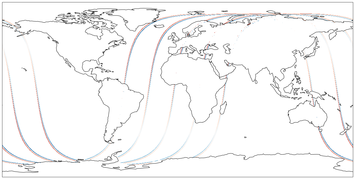
Now let’s plot a variable (ssh_karin) from these 10 files in a chosen projection.
Access Files without any Downloads to your running instance
We can also do that same plot without ‘downloading’ the data to our cloud instance (i.e. disk) first. Let’s try accessing the data from S3 directly through xarray (Xarray is a python package for working with labeled multi-dimensional (a.k.a. N-dimensional, ND) arrays).
CPU times: user 5.58 s, sys: 367 ms, total: 5.95 s
Wall time: 11.4 s<xarray.Dataset>
Dimensions: (num_lines: 88796, num_pixels: 71,
num_sides: 2)
Coordinates:
latitude (num_lines, num_pixels) float64 dask.array<chunksize=(9866, 71), meta=np.ndarray>
longitude (num_lines, num_pixels) float64 dask.array<chunksize=(9866, 71), meta=np.ndarray>
latitude_nadir (num_lines) float64 dask.array<chunksize=(9866,), meta=np.ndarray>
longitude_nadir (num_lines) float64 dask.array<chunksize=(9866,), meta=np.ndarray>
Dimensions without coordinates: num_lines, num_pixels, num_sides
Data variables: (12/91)
time (num_lines) float64 dask.array<chunksize=(9866,), meta=np.ndarray>
time_tai (num_lines) float64 dask.array<chunksize=(9866,), meta=np.ndarray>
ssh_karin (num_lines, num_pixels) float64 dask.array<chunksize=(9866, 71), meta=np.ndarray>
ssh_karin_uncert (num_lines, num_pixels) float32 dask.array<chunksize=(9866, 71), meta=np.ndarray>
ssha_karin (num_lines, num_pixels) float64 dask.array<chunksize=(9866, 71), meta=np.ndarray>
ssh_karin_2 (num_lines, num_pixels) float64 dask.array<chunksize=(9866, 71), meta=np.ndarray>
... ...
simulated_error_baseline_dilation (num_lines, num_pixels) float64 dask.array<chunksize=(9866, 71), meta=np.ndarray>
simulated_error_timing (num_lines, num_pixels) float64 dask.array<chunksize=(9866, 71), meta=np.ndarray>
simulated_error_roll (num_lines, num_pixels) float64 dask.array<chunksize=(9866, 71), meta=np.ndarray>
simulated_error_phase (num_lines, num_pixels) float64 dask.array<chunksize=(9866, 71), meta=np.ndarray>
simulated_error_orbital (num_lines, num_pixels) float64 dask.array<chunksize=(9866, 71), meta=np.ndarray>
simulated_error_karin (num_lines, num_pixels) float64 dask.array<chunksize=(9866, 71), meta=np.ndarray>
Attributes: (12/32)
Conventions: CF-1.7
title: Level 2 Low Rate Sea Surface Height Data Prod...
institution: CNES/JPL
source: Simulate product
history: 2021-09-10 09:54:55Z : Creation
platform: SWOT
... ...
right_last_longitude: 131.81928697472432
right_last_latitude: 77.03254381435897
wavelength: 0.008385803020979
orbit_solution: POE
ellipsoid_semi_major_axis: 6378137.0
ellipsoid_flattening: 0.003352810664781205xarray.Dataset
- num_lines: 88796
- num_pixels: 71
- num_sides: 2
- latitude(num_lines, num_pixels)float64dask.array<chunksize=(9866, 71), meta=np.ndarray>
- long_name :
- latitude (positive N, negative S)
- standard_name :
- latitude
- units :
- degrees_north
- valid_min :
- -80000000
- valid_max :
- 80000000
- comment :
- Latitude of measurement [-80,80]. Positive latitude is North latitude, negative latitude is South latitude.
Array Chunk Bytes 48.10 MiB 5.35 MiB Shape (88796, 71) (9869, 71) Count 27 Tasks 9 Chunks Type float64 numpy.ndarray - longitude(num_lines, num_pixels)float64dask.array<chunksize=(9866, 71), meta=np.ndarray>
- long_name :
- longitude (degrees East)
- standard_name :
- longitude
- units :
- degrees_east
- valid_min :
- 0
- valid_max :
- 359999999
- comment :
- Longitude of measurement. East longitude relative to Greenwich meridian.
Array Chunk Bytes 48.10 MiB 5.35 MiB Shape (88796, 71) (9869, 71) Count 27 Tasks 9 Chunks Type float64 numpy.ndarray - latitude_nadir(num_lines)float64dask.array<chunksize=(9866,), meta=np.ndarray>
- long_name :
- latitude of satellite nadir point
- standard_name :
- latitude
- units :
- degrees_north
- valid_min :
- -80000000
- valid_max :
- 80000000
- comment :
- Geodetic latitude [-80,80] (degrees north of equator) of the satellite nadir point.
Array Chunk Bytes 693.72 kiB 77.10 kiB Shape (88796,) (9869,) Count 27 Tasks 9 Chunks Type float64 numpy.ndarray - longitude_nadir(num_lines)float64dask.array<chunksize=(9866,), meta=np.ndarray>
- long_name :
- longitude of satellite nadir point
- standard_name :
- longitude
- units :
- degrees_east
- valid_min :
- 0
- valid_max :
- 359999999
- comment :
- Longitude (degrees east of Grenwich meridian) of the satellite nadir point.
Array Chunk Bytes 693.72 kiB 77.10 kiB Shape (88796,) (9869,) Count 27 Tasks 9 Chunks Type float64 numpy.ndarray
- time(num_lines)float64dask.array<chunksize=(9866,), meta=np.ndarray>
- long_name :
- time in UTC
- standard_name :
- time
- calendar :
- gregorian
- leap_second :
- YYYY-MM-DDThh:mm:ssZ
- units :
- seconds since 2000-01-01 00:00:00.0
- comment :
- Time of measurement in seconds in the UTC time scale since 1 Jan 2000 00:00:00 UTC. [tai_utc_difference] is the difference between TAI and UTC reference time (seconds) for the first measurement of the data set. If a leap second occurs within the data set, the attribute leap_second is set to the UTC time at which the leap second occurs.
- tai_utc_difference :
- 35.0
Array Chunk Bytes 693.72 kiB 77.10 kiB Shape (88796,) (9869,) Count 27 Tasks 9 Chunks Type float64 numpy.ndarray - time_tai(num_lines)float64dask.array<chunksize=(9866,), meta=np.ndarray>
- long_name :
- time in TAI
- standard_name :
- time
- calendar :
- gregorian
- tai_utc_difference :
- [Value of TAI-UTC at time of first record]
- units :
- seconds since 2000-01-01 00:00:00.0
- comment :
- Time of measurement in seconds in the TAI time scale since 1 Jan 2000 00:00:00 TAI. This time scale contains no leap seconds. The difference (in seconds) with time in UTC is given by the attribute [time:tai_utc_difference].
Array Chunk Bytes 693.72 kiB 77.10 kiB Shape (88796,) (9869,) Count 27 Tasks 9 Chunks Type float64 numpy.ndarray - ssh_karin(num_lines, num_pixels)float64dask.array<chunksize=(9866, 71), meta=np.ndarray>
- long_name :
- sea surface height
- standard_name :
- sea surface height above reference ellipsoid
- units :
- m
- valid_min :
- -15000000
- valid_max :
- 150000000
- comment :
- Fully corrected sea surface height measured by KaRIn. The height is relative to the reference ellipsoid defined in the global attributes. This value is computed using radiometer measurements for wet troposphere effects on the KaRIn measurement (e.g., rad_wet_tropo_cor and sea_state_bias_cor).
Array Chunk Bytes 48.10 MiB 5.35 MiB Shape (88796, 71) (9869, 71) Count 27 Tasks 9 Chunks Type float64 numpy.ndarray - ssh_karin_uncert(num_lines, num_pixels)float32dask.array<chunksize=(9866, 71), meta=np.ndarray>
- long_name :
- sea surface height anomaly uncertainty
- units :
- m
- valid_min :
- 0
- valid_max :
- 60000
- comment :
- 1-sigma uncertainty on the sea surface height from the KaRIn measurement.
Array Chunk Bytes 24.05 MiB 2.67 MiB Shape (88796, 71) (9869, 71) Count 27 Tasks 9 Chunks Type float32 numpy.ndarray - ssha_karin(num_lines, num_pixels)float64dask.array<chunksize=(9866, 71), meta=np.ndarray>
- long_name :
- sea surface height anomaly
- units :
- m
- valid_min :
- -1000000
- valid_max :
- 1000000
- comment :
- Sea surface height anomaly from the KaRIn measurement = ssh_karin - mean_sea_surface_cnescls - solid_earth_tide - ocean_tide_fes – internal_tide_hret - pole_tide - dac.
Array Chunk Bytes 48.10 MiB 5.35 MiB Shape (88796, 71) (9869, 71) Count 27 Tasks 9 Chunks Type float64 numpy.ndarray - ssh_karin_2(num_lines, num_pixels)float64dask.array<chunksize=(9866, 71), meta=np.ndarray>
- long_name :
- sea surface height
- standard_name :
- sea surface height above reference ellipsoid
- units :
- m
- valid_min :
- -15000000
- valid_max :
- 150000000
- comment :
- Fully corrected sea surface height measured by KaRIn. The height is relative to the reference ellipsoid defined in the global attributes. This value is computed using model-based estimates for wet troposphere effects on the KaRIn measurement (e.g., model_wet_tropo_cor and sea_state_bias_cor_2).
Array Chunk Bytes 48.10 MiB 5.35 MiB Shape (88796, 71) (9869, 71) Count 27 Tasks 9 Chunks Type float64 numpy.ndarray - ssha_karin_2(num_lines, num_pixels)float64dask.array<chunksize=(9866, 71), meta=np.ndarray>
- long_name :
- sea surface height anomaly
- units :
- m
- valid_min :
- -1000000
- valid_max :
- 1000000
- comment :
- Sea surface height anomaly from the KaRIn measurement = ssh_karin_2 - mean_sea_surface_cnescls - solid_earth_tide - ocean_tide_fes – internal_tide_hret - pole_tide - dac.
Array Chunk Bytes 48.10 MiB 5.35 MiB Shape (88796, 71) (9869, 71) Count 27 Tasks 9 Chunks Type float64 numpy.ndarray - ssha_karin_qual(num_lines, num_pixels)float64dask.array<chunksize=(9866, 71), meta=np.ndarray>
- long_name :
- sea surface height quality flag
- standard_name :
- status_flag
- flag_meanings :
- good bad
- flag_values :
- [0 1]
- valid_min :
- 0
- valid_max :
- 1
- comment :
- Quality flag for the SSHA from KaRIn.
Array Chunk Bytes 48.10 MiB 5.35 MiB Shape (88796, 71) (9869, 71) Count 27 Tasks 9 Chunks Type float64 numpy.ndarray - polarization_karin(num_lines, num_sides)objectdask.array<chunksize=(9866, 2), meta=np.ndarray>
- long_name :
- polarization for each side of the KaRIn swath
- comment :
- H denotes co-polarized linear horizontal, V denotes co-polarized linear vertical.
Array Chunk Bytes 1.35 MiB 154.20 kiB Shape (88796, 2) (9869, 2) Count 27 Tasks 9 Chunks Type object numpy.ndarray - swh_karin(num_lines, num_pixels)float32dask.array<chunksize=(9866, 71), meta=np.ndarray>
- long_name :
- significant wave height from KaRIn
- standard_name :
- sea_surface_wave_significant_height
- units :
- m
- valid_min :
- 0
- valid_max :
- 25000
- comment :
- Significant wave height from KaRIn volumetric correlation.
Array Chunk Bytes 24.05 MiB 2.67 MiB Shape (88796, 71) (9869, 71) Count 27 Tasks 9 Chunks Type float32 numpy.ndarray - swh_karin_uncert(num_lines, num_pixels)float32dask.array<chunksize=(9866, 71), meta=np.ndarray>
- long_name :
- 1-sigma uncertainty on significant wave height from KaRIn
- units :
- m
- valid_min :
- 0
- valid_max :
- 25000
- comment :
- 1-sigma uncertainty on significant wave height from KaRIn.
Array Chunk Bytes 24.05 MiB 2.67 MiB Shape (88796, 71) (9869, 71) Count 27 Tasks 9 Chunks Type float32 numpy.ndarray - sig0_karin(num_lines, num_pixels)float32dask.array<chunksize=(9866, 71), meta=np.ndarray>
- long_name :
- normalized radar cross section (sigma0) from KaRIn
- standard_name :
- surface_backwards_scattering_coefficient_of_radar_wave
- units :
- 1
- valid_min :
- -1000.0
- valid_max :
- 10000000.0
- comment :
- Normalized radar cross section (sigma0) from KaRIn in real, linear units (not decibels). The value may be negative due to noise subtraction. The value is corrected for instrument calibration and atmospheric attenuation. Radiometer measurements provide the atmospheric attenuation (sig0_cor_atmos_rad).
Array Chunk Bytes 24.05 MiB 2.67 MiB Shape (88796, 71) (9869, 71) Count 27 Tasks 9 Chunks Type float32 numpy.ndarray - sig0_karin_uncert(num_lines, num_pixels)float32dask.array<chunksize=(9866, 71), meta=np.ndarray>
- long_name :
- 1-sigma uncertainty on sigma0 from KaRIn
- units :
- 1
- valid_min :
- 0.0
- valid_max :
- 1000.0
- comment :
- 1-sigma uncertainty on sigma0 from KaRIn.
Array Chunk Bytes 24.05 MiB 2.67 MiB Shape (88796, 71) (9869, 71) Count 27 Tasks 9 Chunks Type float32 numpy.ndarray - sig0_karin_2(num_lines, num_pixels)float32dask.array<chunksize=(9866, 71), meta=np.ndarray>
- long_name :
- normalized radar cross section (sigma0) from KaRIn
- standard_name :
- surface_backwards_scattering_coefficient_of_radar_wave
- units :
- 1
- valid_min :
- -1000.0
- valid_max :
- 10000000.0
- comment :
- Normalized radar cross section (sigma0) from KaRIn in real, linear units (not decibels). The value may be negative due to noise subtraction. The value is corrected for instrument calibration and atmospheric attenuation. A meteorological model provides the atmospheric attenuation (sig0_cor_atmos_model).
Array Chunk Bytes 24.05 MiB 2.67 MiB Shape (88796, 71) (9869, 71) Count 27 Tasks 9 Chunks Type float32 numpy.ndarray - wind_speed_karin(num_lines, num_pixels)float32dask.array<chunksize=(9866, 71), meta=np.ndarray>
- long_name :
- wind speed from KaRIn
- standard_name :
- wind_speed
- source :
- TBD
- units :
- m/s
- valid_min :
- 0
- valid_max :
- 65000
- comment :
- Wind speed from KaRIn computed from sig0_karin.
Array Chunk Bytes 24.05 MiB 2.67 MiB Shape (88796, 71) (9869, 71) Count 27 Tasks 9 Chunks Type float32 numpy.ndarray - wind_speed_karin_2(num_lines, num_pixels)float32dask.array<chunksize=(9866, 71), meta=np.ndarray>
- long_name :
- wind speed from KaRIn
- standard_name :
- wind_speed
- source :
- TBD
- units :
- m/s
- valid_min :
- 0
- valid_max :
- 65000
- comment :
- Wind speed from KaRIn computed from sig0_karin_2.
Array Chunk Bytes 24.05 MiB 2.67 MiB Shape (88796, 71) (9869, 71) Count 27 Tasks 9 Chunks Type float32 numpy.ndarray - swh_karin_qual(num_lines, num_pixels)float64dask.array<chunksize=(9866, 71), meta=np.ndarray>
- long_name :
- quality flag for significant wave height from KaRIn.
- standard_name :
- status_flag
- flag_meanings :
- good bad
- flag_values :
- [0 1]
- valid_min :
- 0
- valid_max :
- 1
- comment :
- Quality flag for significant wave height from KaRIn.
Array Chunk Bytes 48.10 MiB 5.35 MiB Shape (88796, 71) (9869, 71) Count 27 Tasks 9 Chunks Type float64 numpy.ndarray - sig0_karin_qual(num_lines, num_pixels)float64dask.array<chunksize=(9866, 71), meta=np.ndarray>
- long_name :
- quality flag for sigma0 from KaRIn.
- standard_name :
- status_flag
- flag_meanings :
- good bad
- flag_values :
- [0 1]
- valid_min :
- 0
- valid_max :
- 1
- comment :
- Quality flag for sigma0 from KaRIn.
Array Chunk Bytes 48.10 MiB 5.35 MiB Shape (88796, 71) (9869, 71) Count 27 Tasks 9 Chunks Type float64 numpy.ndarray - num_pt_avg(num_lines, num_pixels)float32dask.array<chunksize=(9866, 71), meta=np.ndarray>
- long_name :
- number of samples averaged
- units :
- 1
- valid_min :
- 0
- valid_max :
- 289
- comment :
- Number of native unsmoothed, beam-combined KaRIn samples averaged.
Array Chunk Bytes 24.05 MiB 2.67 MiB Shape (88796, 71) (9869, 71) Count 27 Tasks 9 Chunks Type float32 numpy.ndarray - swh_model(num_lines, num_pixels)float32dask.array<chunksize=(9866, 71), meta=np.ndarray>
- long_name :
- significant wave height from wave model
- standard_name :
- sea_surface_wave_significant_height
- source :
- European Centre for Medium-Range Weather Forecasts
- institution :
- ECMWF
- units :
- m
- valid_min :
- 0
- valid_max :
- 30000
- comment :
- Significant wave height from model.
Array Chunk Bytes 24.05 MiB 2.67 MiB Shape (88796, 71) (9869, 71) Count 27 Tasks 9 Chunks Type float32 numpy.ndarray - mean_wave_direction(num_lines, num_pixels)float32dask.array<chunksize=(9866, 71), meta=np.ndarray>
- long_name :
- mean sea surface wave direction
- source :
- Meteo France Wave Model (MF-WAM)
- institution :
- Meteo France
- units :
- degree
- valid_min :
- 0
- valid_max :
- 36000
- comment :
- Mean sea surface wave direction.
Array Chunk Bytes 24.05 MiB 2.67 MiB Shape (88796, 71) (9869, 71) Count 27 Tasks 9 Chunks Type float32 numpy.ndarray - mean_wave_period_t02(num_lines, num_pixels)float32dask.array<chunksize=(9866, 71), meta=np.ndarray>
- long_name :
- sea surface wind wave mean period
- standard_name :
- sea_surface_wave_significant_period
- source :
- Meteo France Wave Model (MF-WAM)
- institution :
- Meteo France
- units :
- s
- valid_min :
- 0
- valid_max :
- 100
- comment :
- Sea surface wind wave mean period from model spectral density second moment.
Array Chunk Bytes 24.05 MiB 2.67 MiB Shape (88796, 71) (9869, 71) Count 27 Tasks 9 Chunks Type float32 numpy.ndarray - wind_speed_model_u(num_lines, num_pixels)float32dask.array<chunksize=(9866, 71), meta=np.ndarray>
- long_name :
- u component of model wind
- standard_name :
- eastward_wind
- source :
- European Centre for Medium-Range Weather Forecasts
- institution :
- ECMWF
- units :
- m/s
- valid_min :
- -30000
- valid_max :
- 30000
- comment :
- Eastward component of the atmospheric model wind vector at 10 meters.
Array Chunk Bytes 24.05 MiB 2.67 MiB Shape (88796, 71) (9869, 71) Count 27 Tasks 9 Chunks Type float32 numpy.ndarray - wind_speed_model_v(num_lines, num_pixels)float32dask.array<chunksize=(9866, 71), meta=np.ndarray>
- long_name :
- v component of model wind
- standard_name :
- northward_wind
- source :
- European Centre for Medium-Range Weather Forecasts
- institution :
- ECMWF
- units :
- m/s
- valid_min :
- -30000
- valid_max :
- 30000
- comment :
- Northward component of the atmospheric model wind vector at 10 meters.
Array Chunk Bytes 24.05 MiB 2.67 MiB Shape (88796, 71) (9869, 71) Count 27 Tasks 9 Chunks Type float32 numpy.ndarray - wind_speed_rad(num_lines, num_sides)float32dask.array<chunksize=(9866, 2), meta=np.ndarray>
- long_name :
- wind speed from radiometer
- standard_name :
- wind_speed
- source :
- Advanced Microwave Radiometer
- units :
- m/s
- valid_min :
- 0
- valid_max :
- 65000
- comment :
- Wind speed from radiometer measurements.
Array Chunk Bytes 693.72 kiB 77.10 kiB Shape (88796, 2) (9869, 2) Count 27 Tasks 9 Chunks Type float32 numpy.ndarray - distance_to_coast(num_lines, num_pixels)float32dask.array<chunksize=(9866, 71), meta=np.ndarray>
- long_name :
- distance to coast
- source :
- MODIS/GlobCover
- institution :
- European Space Agency
- units :
- m
- valid_min :
- 0
- valid_max :
- 21000
- comment :
- Approximate distance to the nearest coast point along the Earth surface.
Array Chunk Bytes 24.05 MiB 2.67 MiB Shape (88796, 71) (9869, 71) Count 27 Tasks 9 Chunks Type float32 numpy.ndarray - heading_to_coast(num_lines, num_pixels)float32dask.array<chunksize=(9866, 71), meta=np.ndarray>
- long_name :
- heading to coast
- units :
- degrees
- valid_min :
- 0
- valid_max :
- 35999
- comment :
- Approximate compass heading (0-360 degrees with respect to true north) to the nearest coast point.
Array Chunk Bytes 24.05 MiB 2.67 MiB Shape (88796, 71) (9869, 71) Count 27 Tasks 9 Chunks Type float32 numpy.ndarray - ancillary_surface_classification_flag(num_lines, num_pixels)float32dask.array<chunksize=(9866, 71), meta=np.ndarray>
- long_name :
- surface classification
- standard_name :
- status_flag
- source :
- MODIS/GlobCover
- institution :
- European Space Agency
- flag_meanings :
- open_ocean land continental_water aquatic_vegetation continental_ice_snow floating_ice salted_basin
- flag_values :
- [0 1 2 3 4 5 6]
- valid_min :
- 0
- valid_max :
- 6
- comment :
- 7-state surface type classification computed from a mask built with MODIS and GlobCover data.
Array Chunk Bytes 24.05 MiB 2.67 MiB Shape (88796, 71) (9869, 71) Count 27 Tasks 9 Chunks Type float32 numpy.ndarray - dynamic_ice_flag(num_lines, num_pixels)float32dask.array<chunksize=(9866, 71), meta=np.ndarray>
- long_name :
- dynamic ice flag
- standard_name :
- status_flag
- source :
- EUMETSAT Ocean and Sea Ice Satellite Applications Facility
- institution :
- EUMETSAT
- flag_meanings :
- no_ice probable_ice ice
- flag_values :
- [0 1 2]
- valid_min :
- 0
- valid_max :
- 2
- comment :
- Dynamic ice flag for the location of the KaRIn measurement.
Array Chunk Bytes 24.05 MiB 2.67 MiB Shape (88796, 71) (9869, 71) Count 27 Tasks 9 Chunks Type float32 numpy.ndarray - rain_flag(num_lines, num_pixels)float32dask.array<chunksize=(9866, 71), meta=np.ndarray>
- long_name :
- rain flag
- standard_name :
- status_flag
- flag_meanings :
- no_rain probable_rain rain
- flag_values :
- [0 1 2]
- valid_min :
- 0
- valid_max :
- 2
- comment :
- Flag indicates that signal is attenuated, probably from rain.
Array Chunk Bytes 24.05 MiB 2.67 MiB Shape (88796, 71) (9869, 71) Count 27 Tasks 9 Chunks Type float32 numpy.ndarray - rad_surface_type_flag(num_lines, num_sides)float32dask.array<chunksize=(9866, 2), meta=np.ndarray>
- long_name :
- radiometer surface type flag
- standard_name :
- status_flag
- source :
- Advanced Microwave Radiometer
- flag_meanings :
- open_ocean coastal_ocean land
- flag_values :
- [0 1 2]
- valid_min :
- 0
- valid_max :
- 2
- comment :
- Flag indicating the validity and type of processing applied to generate the wet troposphere correction (rad_wet_tropo_cor). A value of 0 indicates that open ocean processing is used, a value of 1 indicates coastal processing, and a value of 2 indicates that rad_wet_tropo_cor is invalid due to land contamination.
Array Chunk Bytes 693.72 kiB 77.10 kiB Shape (88796, 2) (9869, 2) Count 27 Tasks 9 Chunks Type float32 numpy.ndarray - sc_altitude(num_lines)float64dask.array<chunksize=(9866,), meta=np.ndarray>
- long_name :
- altitude of KMSF origin
- standard_name :
- height_above_reference_ellipsoid
- units :
- m
- valid_min :
- 0
- valid_max :
- 2000000000
- comment :
- Altitude of the KMSF origin.
Array Chunk Bytes 693.72 kiB 77.10 kiB Shape (88796,) (9869,) Count 27 Tasks 9 Chunks Type float64 numpy.ndarray - orbit_alt_rate(num_lines)float32dask.array<chunksize=(9866,), meta=np.ndarray>
- long_name :
- orbital altitude rate with respect to mean sea surface
- units :
- m/s
- valid_min :
- -3500
- valid_max :
- 3500
- comment :
- Orbital altitude rate with respect to the mean sea surface.
Array Chunk Bytes 346.86 kiB 38.55 kiB Shape (88796,) (9869,) Count 27 Tasks 9 Chunks Type float32 numpy.ndarray - cross_track_angle(num_lines)float64dask.array<chunksize=(9866,), meta=np.ndarray>
- long_name :
- cross-track angle from true north
- units :
- degrees
- valid_min :
- 0
- valid_max :
- 359999999
- comment :
- Angle with respect to true north of the cross-track direction to the right of the spacecraft velocity vector.
Array Chunk Bytes 693.72 kiB 77.10 kiB Shape (88796,) (9869,) Count 27 Tasks 9 Chunks Type float64 numpy.ndarray - sc_roll(num_lines)float64dask.array<chunksize=(9866,), meta=np.ndarray>
- long_name :
- roll of the spacecraft
- standard_name :
- platform_roll_angle
- units :
- degrees
- valid_min :
- -1799999
- valid_max :
- 1800000
- comment :
- KMSF attitude roll angle; positive values move the +y antenna down.
Array Chunk Bytes 693.72 kiB 77.10 kiB Shape (88796,) (9869,) Count 27 Tasks 9 Chunks Type float64 numpy.ndarray - sc_pitch(num_lines)float64dask.array<chunksize=(9866,), meta=np.ndarray>
- long_name :
- pitch of the spacecraft
- standard_name :
- platform_pitch_angle
- units :
- degrees
- valid_min :
- -1799999
- valid_max :
- 1800000
- comment :
- KMSF attitude pitch angle; positive values move the KMSF +x axis up.
Array Chunk Bytes 693.72 kiB 77.10 kiB Shape (88796,) (9869,) Count 27 Tasks 9 Chunks Type float64 numpy.ndarray - sc_yaw(num_lines)float64dask.array<chunksize=(9866,), meta=np.ndarray>
- long_name :
- yaw of the spacecraft
- standard_name :
- platform_yaw_angle
- units :
- degrees
- valid_min :
- -1799999
- valid_max :
- 1800000
- comment :
- KMSF attitude yaw angle relative to the nadir track. The yaw angle is a right-handed rotation about the nadir (downward) direction. A yaw value of 0 deg indicates that the KMSF +x axis is aligned with the horizontal component of the Earth-relative velocity vector. A yaw value of 180 deg indicates that the spacecraft is in a yaw-flipped state, with the KMSF -x axis aligned with the horizontal component of the Earth-relative velocity vector.
Array Chunk Bytes 693.72 kiB 77.10 kiB Shape (88796,) (9869,) Count 27 Tasks 9 Chunks Type float64 numpy.ndarray - velocity_heading(num_lines)float64dask.array<chunksize=(9866,), meta=np.ndarray>
- long_name :
- heading of the spacecraft Earth-relative velocity vector
- units :
- degrees
- valid_min :
- 0
- valid_max :
- 359999999
- comment :
- Angle with respect to true north of the horizontal component of the spacecraft Earth-relative velocity vector. A value of 90 deg indicates that the spacecraft velocity vector pointed due east. Values between 0 and 90 deg indicate that the velocity vector has a northward component, and values between 90 and 180 deg indicate that the velocity vector has a southward component.
Array Chunk Bytes 693.72 kiB 77.10 kiB Shape (88796,) (9869,) Count 27 Tasks 9 Chunks Type float64 numpy.ndarray - orbit_qual(num_lines)float32dask.array<chunksize=(9866,), meta=np.ndarray>
- long_name :
- orbit quality flag
- standard_name :
- status_flag
- valid_min :
- 0
- valid_max :
- 1
- comment :
- Orbit quality flag.
Array Chunk Bytes 346.86 kiB 38.55 kiB Shape (88796,) (9869,) Count 27 Tasks 9 Chunks Type float32 numpy.ndarray - latitude_avg_ssh(num_lines, num_pixels)float64dask.array<chunksize=(9866, 71), meta=np.ndarray>
- long_name :
- weighted average latitude of samples used to compute SSH
- standard_name :
- latitude
- units :
- degrees_north
- valid_min :
- -80000000
- valid_max :
- 80000000
- comment :
- Latitude of measurement [-80,80]. Positive latitude is North latitude, negative latitude is South latitude. This value may be biased away from a nominal grid location if some of the native, unsmoothed samples were discarded during processing.
Array Chunk Bytes 48.10 MiB 5.35 MiB Shape (88796, 71) (9869, 71) Count 27 Tasks 9 Chunks Type float64 numpy.ndarray - longitude_avg_ssh(num_lines, num_pixels)float64dask.array<chunksize=(9866, 71), meta=np.ndarray>
- long_name :
- weighted average longitude of samples used to compute SSH
- standard_name :
- longitude
- units :
- degrees_east
- valid_min :
- 0
- valid_max :
- 359999999
- comment :
- Longitude of measurement. East longitude relative to Greenwich meridian. This value may be biased away from a nominal grid location if some of the native, unsmoothed samples were discarded during processing.
Array Chunk Bytes 48.10 MiB 5.35 MiB Shape (88796, 71) (9869, 71) Count 27 Tasks 9 Chunks Type float64 numpy.ndarray - cross_track_distance(num_lines, num_pixels)float32dask.array<chunksize=(9866, 71), meta=np.ndarray>
- long_name :
- cross track distance
- units :
- m
- valid_min :
- -75000.0
- valid_max :
- 75000.0
- comment :
- Distance of sample from nadir. Negative values indicate the left side of the swath, and positive values indicate the right side of the swath.
Array Chunk Bytes 24.05 MiB 2.67 MiB Shape (88796, 71) (9869, 71) Count 27 Tasks 9 Chunks Type float32 numpy.ndarray - x_factor(num_lines, num_pixels)float32dask.array<chunksize=(9866, 71), meta=np.ndarray>
- long_name :
- radiometric calibration X factor as a composite value for the X factors of the +y and -y channels
- units :
- 1
- valid_min :
- 0.0
- valid_max :
- 1e+20
- comment :
- Radiometric calibration X factor as a linear power ratio.
Array Chunk Bytes 24.05 MiB 2.67 MiB Shape (88796, 71) (9869, 71) Count 27 Tasks 9 Chunks Type float32 numpy.ndarray - sig0_cor_atmos_model(num_lines, num_pixels)float32dask.array<chunksize=(9866, 71), meta=np.ndarray>
- long_name :
- two-way atmospheric correction to sigma0 from model
- source :
- European Centre for Medium-Range Weather Forecasts
- institution :
- ECMWF
- units :
- 1
- valid_min :
- 1.0
- valid_max :
- 10.0
- comment :
- Atmospheric correction to sigma0 from weather model data as a linear power multiplier (not decibels). sig0_cor_atmos_model is already applied in computing sig0_karin_2.
Array Chunk Bytes 24.05 MiB 2.67 MiB Shape (88796, 71) (9869, 71) Count 27 Tasks 9 Chunks Type float32 numpy.ndarray - sig0_cor_atmos_rad(num_lines, num_pixels)float32dask.array<chunksize=(9866, 71), meta=np.ndarray>
- long_name :
- two-way atmospheric correction to sigma0 from radiometer data
- source :
- Advanced Microwave Radiometer
- units :
- 1
- valid_min :
- 1.0
- valid_max :
- 10.0
- comment :
- Atmospheric correction to sigma0 from radiometer data as a linear power multiplier (not decibels). sig0_cor_atmos_rad is already applied in computing sig0_karin.
Array Chunk Bytes 24.05 MiB 2.67 MiB Shape (88796, 71) (9869, 71) Count 27 Tasks 9 Chunks Type float32 numpy.ndarray - doppler_centroid(num_lines, num_sides)float32dask.array<chunksize=(9866, 2), meta=np.ndarray>
- long_name :
- doppler centroid estimated by KaRIn
- units :
- 1/s
- valid_min :
- -30000
- valid_max :
- 30000
- comment :
- Doppler centroid (in hertz or cycles per second) estimated by KaRIn.
Array Chunk Bytes 693.72 kiB 77.10 kiB Shape (88796, 2) (9869, 2) Count 27 Tasks 9 Chunks Type float32 numpy.ndarray - phase_bias_ref_surface(num_lines, num_pixels)float64dask.array<chunksize=(9866, 71), meta=np.ndarray>
- long_name :
- height of reference surface used for phase bias calculation
- units :
- m
- valid_min :
- -15000000
- valid_max :
- 150000000
- comment :
- Height (relative to the reference ellipsoid) of the reference surface used for phase bias calculation during L1B processing.
Array Chunk Bytes 48.10 MiB 5.35 MiB Shape (88796, 71) (9869, 71) Count 27 Tasks 9 Chunks Type float64 numpy.ndarray - obp_ref_surface(num_lines, num_pixels)float64dask.array<chunksize=(9866, 71), meta=np.ndarray>
- long_name :
- height of reference surface used by on-board-processor
- units :
- m
- valid_min :
- -15000000
- valid_max :
- 150000000
- comment :
- Height (relative to the reference ellipsoid) of the reference surface used by the KaRIn on-board processor.
Array Chunk Bytes 48.10 MiB 5.35 MiB Shape (88796, 71) (9869, 71) Count 27 Tasks 9 Chunks Type float64 numpy.ndarray - rad_tmb_187(num_lines, num_sides)float32dask.array<chunksize=(9866, 2), meta=np.ndarray>
- long_name :
- radiometer main beam brightness temperature at 18.7 GHz
- standard_name :
- toa_brightness_temperature
- source :
- Advanced Microwave Radiometer
- units :
- K
- valid_min :
- 13000
- valid_max :
- 25000
- comment :
- Main beam brightness temperature measurement at 18.7 GHz. Value is unsmoothed (along-track averaging has not been performed).
Array Chunk Bytes 693.72 kiB 77.10 kiB Shape (88796, 2) (9869, 2) Count 27 Tasks 9 Chunks Type float32 numpy.ndarray - rad_tmb_238(num_lines, num_sides)float32dask.array<chunksize=(9866, 2), meta=np.ndarray>
- long_name :
- radiometer main beam brightness temperature at 23.8 GHz
- standard_name :
- toa_brightness_temperature
- source :
- Advanced Microwave Radiometer
- units :
- K
- valid_min :
- 13000
- valid_max :
- 25000
- comment :
- Main beam brightness temperature measurement at 23.8 GHz. Value is unsmoothed (along-track averaging has not been performed).
Array Chunk Bytes 693.72 kiB 77.10 kiB Shape (88796, 2) (9869, 2) Count 27 Tasks 9 Chunks Type float32 numpy.ndarray - rad_tmb_340(num_lines, num_sides)float32dask.array<chunksize=(9866, 2), meta=np.ndarray>
- long_name :
- radiometer main beam brightness temperature at 34.0 GHz
- standard_name :
- toa_brightness_temperature
- source :
- Advanced Microwave Radiometer
- units :
- K
- valid_min :
- 15000
- valid_max :
- 28000
- comment :
- Main beam brightness temperature measurement at 34.0 GHz. Value is unsmoothed (along-track averaging has not been performed).
Array Chunk Bytes 693.72 kiB 77.10 kiB Shape (88796, 2) (9869, 2) Count 27 Tasks 9 Chunks Type float32 numpy.ndarray - rad_water_vapor(num_lines, num_sides)float32dask.array<chunksize=(9866, 2), meta=np.ndarray>
- long_name :
- water vapor content from radiometer
- standard_name :
- atmosphere_water_vapor_content
- source :
- Advanced Microwave Radiometer
- units :
- kg/m^2
- valid_min :
- 0
- valid_max :
- 15000
- comment :
- Integrated water vapor content from radiometer measurements.
Array Chunk Bytes 693.72 kiB 77.10 kiB Shape (88796, 2) (9869, 2) Count 27 Tasks 9 Chunks Type float32 numpy.ndarray - rad_cloud_liquid_water(num_lines, num_sides)float32dask.array<chunksize=(9866, 2), meta=np.ndarray>
- long_name :
- liquid water content from radiometer
- standard_name :
- atmosphere_cloud_liquid_water_content
- source :
- Advanced Microwave Radiometer
- units :
- kg/m^2
- valid_min :
- 0
- valid_max :
- 2000
- comment :
- Integrated cloud liquid water content from radiometer measurements.
Array Chunk Bytes 693.72 kiB 77.10 kiB Shape (88796, 2) (9869, 2) Count 27 Tasks 9 Chunks Type float32 numpy.ndarray - mean_sea_surface_cnescls(num_lines, num_pixels)float64dask.array<chunksize=(9866, 71), meta=np.ndarray>
- long_name :
- mean sea surface height (CNES/CLS)
- source :
- CNES_CLS_15
- institution :
- CNES/CLS
- units :
- m
- valid_min :
- -1500000
- valid_max :
- 1500000
- comment :
- Mean sea surface height above the reference ellipsoid. The value is referenced to the mean tide system, i.e. includes the permanent tide (zero frequency).
Array Chunk Bytes 48.10 MiB 5.35 MiB Shape (88796, 71) (9869, 71) Count 27 Tasks 9 Chunks Type float64 numpy.ndarray - mean_sea_surface_cnescls_uncert(num_lines, num_pixels)float32dask.array<chunksize=(9866, 71), meta=np.ndarray>
- long_name :
- mean sea surface height accuracy (CNES/CLS)
- source :
- CNES_CLS_15
- institution :
- CNES/CLS
- units :
- m
- valid_min :
- 0
- valid_max :
- 10000
- comment :
- Accuracy of the mean sea surface height (mean_sea_surface_cnescls).
Array Chunk Bytes 24.05 MiB 2.67 MiB Shape (88796, 71) (9869, 71) Count 27 Tasks 9 Chunks Type float32 numpy.ndarray - mean_sea_surface_dtu(num_lines, num_pixels)float64dask.array<chunksize=(9866, 71), meta=np.ndarray>
- long_name :
- mean sea surface height (DTU)
- source :
- DTU18
- institution :
- DTU
- units :
- m
- valid_min :
- -1500000
- valid_max :
- 1500000
- comment :
- Mean sea surface height above the reference ellipsoid. The value is referenced to the mean tide system, i.e. includes the permanent tide (zero frequency).
Array Chunk Bytes 48.10 MiB 5.35 MiB Shape (88796, 71) (9869, 71) Count 27 Tasks 9 Chunks Type float64 numpy.ndarray - mean_sea_surface_dtu_uncert(num_lines, num_pixels)float32dask.array<chunksize=(9866, 71), meta=np.ndarray>
- long_name :
- mean sea surface height accuracy (DTU)
- source :
- DTU18
- institution :
- DTU
- units :
- m
- valid_min :
- 0
- valid_max :
- 10000
- comment :
- Accuracy of the mean sea surface height (mean_sea_surface_dtu)
Array Chunk Bytes 24.05 MiB 2.67 MiB Shape (88796, 71) (9869, 71) Count 27 Tasks 9 Chunks Type float32 numpy.ndarray - geoid(num_lines, num_pixels)float64dask.array<chunksize=(9866, 71), meta=np.ndarray>
- long_name :
- geoid height
- standard_name :
- geoid_height_above_reference_ellipsoid
- source :
- EGM2008 (Pavlis et al., 2012)
- units :
- m
- valid_min :
- -1500000
- valid_max :
- 1500000
- comment :
- Geoid height above the reference ellipsoid with a correction to refer the value to the mean tide system, i.e. includes the permanent tide (zero frequency).
Array Chunk Bytes 48.10 MiB 5.35 MiB Shape (88796, 71) (9869, 71) Count 27 Tasks 9 Chunks Type float64 numpy.ndarray - mean_dynamic_topography(num_lines, num_pixels)float32dask.array<chunksize=(9866, 71), meta=np.ndarray>
- long_name :
- mean dynamic topography
- source :
- CNES_CLS_18
- institution :
- CNES/CLS
- units :
- m
- valid_min :
- -30000
- valid_max :
- 30000
- comment :
- Mean dynamic topography above the geoid.
Array Chunk Bytes 24.05 MiB 2.67 MiB Shape (88796, 71) (9869, 71) Count 27 Tasks 9 Chunks Type float32 numpy.ndarray - mean_dynamic_topography_uncert(num_lines, num_pixels)float32dask.array<chunksize=(9866, 71), meta=np.ndarray>
- long_name :
- mean dynamic topography accuracy
- source :
- CNES_CLS_18
- institution :
- CNES/CLS
- units :
- m
- valid_min :
- 0
- valid_max :
- 10000
- comment :
- Accuracy of the mean dynamic topography.
Array Chunk Bytes 24.05 MiB 2.67 MiB Shape (88796, 71) (9869, 71) Count 27 Tasks 9 Chunks Type float32 numpy.ndarray - depth_or_elevation(num_lines, num_pixels)float32dask.array<chunksize=(9866, 71), meta=np.ndarray>
- long_name :
- ocean depth or land elevation
- source :
- Altimeter Corrected Elevations, version 2
- institution :
- European Space Agency
- units :
- m
- valid_min :
- -12000
- valid_max :
- 10000
- comment :
- Ocean depth or land elevation above reference ellipsoid. Ocean depth (bathymetry) is given as negative values, and land elevation positive values.
Array Chunk Bytes 24.05 MiB 2.67 MiB Shape (88796, 71) (9869, 71) Count 27 Tasks 9 Chunks Type float32 numpy.ndarray - solid_earth_tide(num_lines, num_pixels)float32dask.array<chunksize=(9866, 71), meta=np.ndarray>
- long_name :
- solid Earth tide height
- source :
- Cartwright and Taylor (1971) and Cartwright and Edden (1973)
- units :
- m
- valid_min :
- -10000
- valid_max :
- 10000
- comment :
- Solid-Earth (body) tide height. The zero-frequency permanent tide component is not included.
Array Chunk Bytes 24.05 MiB 2.67 MiB Shape (88796, 71) (9869, 71) Count 27 Tasks 9 Chunks Type float32 numpy.ndarray - ocean_tide_fes(num_lines, num_pixels)float64dask.array<chunksize=(9866, 71), meta=np.ndarray>
- long_name :
- geocentric ocean tide height (FES)
- source :
- FES2014b (Carrere et al., 2016)
- institution :
- LEGOS/CNES
- units :
- m
- valid_min :
- -300000
- valid_max :
- 300000
- comment :
- Geocentric ocean tide height. Includes the sum total of the ocean tide, the corresponding load tide (load_tide_fes) and equilibrium long-period ocean tide height (ocean_tide_eq).
Array Chunk Bytes 48.10 MiB 5.35 MiB Shape (88796, 71) (9869, 71) Count 27 Tasks 9 Chunks Type float64 numpy.ndarray - ocean_tide_got(num_lines, num_pixels)float64dask.array<chunksize=(9866, 71), meta=np.ndarray>
- long_name :
- geocentric ocean tide height (GOT)
- source :
- GOT4.10c (Ray, 2013)
- institution :
- GSFC
- units :
- m
- valid_min :
- -300000
- valid_max :
- 300000
- comment :
- Geocentric ocean tide height. Includes the sum total of the ocean tide, the corresponding load tide (load_tide_got) and equilibrium long-period ocean tide height (ocean_tide_eq).
Array Chunk Bytes 48.10 MiB 5.35 MiB Shape (88796, 71) (9869, 71) Count 27 Tasks 9 Chunks Type float64 numpy.ndarray - load_tide_fes(num_lines, num_pixels)float32dask.array<chunksize=(9866, 71), meta=np.ndarray>
- long_name :
- geocentric load tide height (FES)
- source :
- FES2014b (Carrere et al., 2016)
- institution :
- LEGOS/CNES
- units :
- m
- valid_min :
- -2000
- valid_max :
- 2000
- comment :
- Geocentric load tide height. The effect of the ocean tide loading of the Earth's crust. This value has already been added to the corresponding ocean tide height value (ocean_tide_fes).
Array Chunk Bytes 24.05 MiB 2.67 MiB Shape (88796, 71) (9869, 71) Count 27 Tasks 9 Chunks Type float32 numpy.ndarray - load_tide_got(num_lines, num_pixels)float32dask.array<chunksize=(9866, 71), meta=np.ndarray>
- long_name :
- geocentric load tide height (GOT)
- source :
- GOT4.10c (Ray, 2013)
- institution :
- GSFC
- units :
- m
- valid_min :
- -2000
- valid_max :
- 2000
- comment :
- Geocentric load tide height. The effect of the ocean tide loading of the Earth's crust. This value has already been added to the corresponding ocean tide height value (ocean_tide_got).
Array Chunk Bytes 24.05 MiB 2.67 MiB Shape (88796, 71) (9869, 71) Count 27 Tasks 9 Chunks Type float32 numpy.ndarray - ocean_tide_eq(num_lines, num_pixels)float32dask.array<chunksize=(9866, 71), meta=np.ndarray>
- long_name :
- equilibrium long-period ocean tide height
- units :
- m
- valid_min :
- -2000
- valid_max :
- 2000
- comment :
- Equilibrium long-period ocean tide height. This value has already been added to the corresponding ocean tide height values (ocean_tide_fes and ocean_tide_got).
Array Chunk Bytes 24.05 MiB 2.67 MiB Shape (88796, 71) (9869, 71) Count 27 Tasks 9 Chunks Type float32 numpy.ndarray - ocean_tide_non_eq(num_lines, num_pixels)float32dask.array<chunksize=(9866, 71), meta=np.ndarray>
- long_name :
- non-equilibrium long-period ocean tide height
- source :
- FES2014b (Carrere et al., 2016)
- institution :
- LEGOS/CNES
- units :
- m
- valid_min :
- -2000
- valid_max :
- 2000
- comment :
- Non-equilibrium long-period ocean tide height. This value is reported as a relative displacement with repsect to ocean_tide_eq. This value can be added to ocean_tide_eq, ocean_tide_fes, or ocean_tide_got, or subtracted from ssha_karin and ssha_karin_2, to account for the total long-period ocean tides from equilibrium and non-equilibrium contributions.
Array Chunk Bytes 24.05 MiB 2.67 MiB Shape (88796, 71) (9869, 71) Count 27 Tasks 9 Chunks Type float32 numpy.ndarray - internal_tide_hret(num_lines, num_pixels)float32dask.array<chunksize=(9866, 71), meta=np.ndarray>
- long_name :
- coherent internal tide (HRET)
- source :
- Zaron (2019)
- units :
- m
- valid_min :
- -2000
- valid_max :
- 2000
- comment :
- Coherent internal ocean tide. This value is subtracted from the ssh_karin and ssh_karin_2 to compute ssha_karin and ssha_karin_2, respectively.
Array Chunk Bytes 24.05 MiB 2.67 MiB Shape (88796, 71) (9869, 71) Count 27 Tasks 9 Chunks Type float32 numpy.ndarray - internal_tide_sol2(num_lines, num_pixels)float32dask.array<chunksize=(9866, 71), meta=np.ndarray>
- long_name :
- coherent internal tide (Model 2)
- source :
- TBD
- units :
- m
- valid_min :
- -2000
- valid_max :
- 2000
- comment :
- Coherent internal tide.
Array Chunk Bytes 24.05 MiB 2.67 MiB Shape (88796, 71) (9869, 71) Count 27 Tasks 9 Chunks Type float32 numpy.ndarray - pole_tide(num_lines, num_pixels)float32dask.array<chunksize=(9866, 71), meta=np.ndarray>
- long_name :
- geocentric pole tide height
- source :
- Wahr (1985) and Desai et al. (2015)
- units :
- m
- valid_min :
- -2000
- valid_max :
- 2000
- comment :
- Geocentric pole tide height. The total of the contribution from the solid-Earth (body) pole tide height, the ocean pole tide height, and the load pole tide height (i.e., the effect of the ocean pole tide loading of the Earth's crust).
Array Chunk Bytes 24.05 MiB 2.67 MiB Shape (88796, 71) (9869, 71) Count 27 Tasks 9 Chunks Type float32 numpy.ndarray - dac(num_lines, num_pixels)float32dask.array<chunksize=(9866, 71), meta=np.ndarray>
- long_name :
- dynamic atmospheric correction
- source :
- MOG2D
- institution :
- LEGOS/CNES/CLS
- units :
- m
- valid_min :
- -12000
- valid_max :
- 12000
- comment :
- Model estimate of the effect on sea surface topography due to high frequency air pressure and wind effects and the low-frequency height from inverted barometer effect (inv_bar_cor). This value is subtracted from the ssh_karin and ssh_karin_2 to compute ssha_karin and ssha_karin_2, respectively. Use only one of inv_bar_cor and dac.
Array Chunk Bytes 24.05 MiB 2.67 MiB Shape (88796, 71) (9869, 71) Count 27 Tasks 9 Chunks Type float32 numpy.ndarray - inv_bar_cor(num_lines, num_pixels)float32dask.array<chunksize=(9866, 71), meta=np.ndarray>
- long_name :
- static inverse barometer effect on sea surface height
- units :
- m
- valid_min :
- -2000
- valid_max :
- 2000
- comment :
- Estimate of static effect of atmospheric pressure on sea surface height. Above average pressure lowers sea surface height. Computed by interpolating ECMWF pressure fields in space and time. The value is included in dac. To apply, add dac to ssha_karin and ssha_karin_2 and subtract inv_bar_cor.
Array Chunk Bytes 24.05 MiB 2.67 MiB Shape (88796, 71) (9869, 71) Count 27 Tasks 9 Chunks Type float32 numpy.ndarray - model_dry_tropo_cor(num_lines, num_pixels)float32dask.array<chunksize=(9866, 71), meta=np.ndarray>
- long_name :
- dry troposphere vertical correction
- source :
- European Centre for Medium-Range Weather Forecasts
- institution :
- ECMWF
- units :
- m
- valid_min :
- -30000
- valid_max :
- -15000
- comment :
- Equivalent vertical correction due to dry troposphere delay. The reported sea surface height, latitude and longitude are computed after adding negative media corrections to uncorrected range along slant-range paths, accounting for the differential delay between the two KaRIn antennas. The equivalent vertical correction is computed by applying obliquity factors to the slant-path correction. Adding the reported correction to the reported sea surface height results in the uncorrected sea surface height.
Array Chunk Bytes 24.05 MiB 2.67 MiB Shape (88796, 71) (9869, 71) Count 27 Tasks 9 Chunks Type float32 numpy.ndarray - model_wet_tropo_cor(num_lines, num_pixels)float32dask.array<chunksize=(9866, 71), meta=np.ndarray>
- long_name :
- wet troposphere vertical correction from weather model data
- source :
- European Centre for Medium-Range Weather Forecasts
- institution :
- ECMWF
- units :
- m
- valid_min :
- -10000
- valid_max :
- 0
- comment :
- Equivalent vertical correction due to wet troposphere delay from weather model data. The reported pixel height, latitude and longitude are computed after adding negative media corrections to uncorrected range along slant-range paths, accounting for the differential delay between the two KaRIn antennas. The equivalent vertical correction is computed by applying obliquity factors to the slant-path correction. Adding the reported correction to the reported sea surface height (ssh_karin_2) results in the uncorrected sea surface height.
Array Chunk Bytes 24.05 MiB 2.67 MiB Shape (88796, 71) (9869, 71) Count 27 Tasks 9 Chunks Type float32 numpy.ndarray - rad_wet_tropo_cor(num_lines, num_pixels)float32dask.array<chunksize=(9866, 71), meta=np.ndarray>
- long_name :
- wet troposphere vertical correction from radiometer data
- source :
- Advanced Microwave Radiometer
- units :
- m
- valid_min :
- -10000
- valid_max :
- 0
- comment :
- Equivalent vertical correction due to wet troposphere delay from radiometer measurements. The reported pixel height, latitude and longitude are computed after adding negative media corrections to uncorrected range along slant-range paths, accounting for the differential delay between the two KaRIn antennas. The equivalent vertical correction is computed by applying obliquity factors to the slant-path correction. Adding the reported correction to the reported sea surface height (ssh_karin) results in the uncorrected sea surface height.
Array Chunk Bytes 24.05 MiB 2.67 MiB Shape (88796, 71) (9869, 71) Count 27 Tasks 9 Chunks Type float32 numpy.ndarray - iono_cor_gim_ka(num_lines, num_pixels)float32dask.array<chunksize=(9866, 71), meta=np.ndarray>
- long_name :
- ionosphere vertical correction
- source :
- Global Ionosphere Maps
- institution :
- JPL
- units :
- m
- valid_min :
- -5000
- valid_max :
- 0
- comment :
- Equivalent vertical correction due to ionosphere delay. The reported sea surface height, latitude and longitude are computed after adding negative media corrections to uncorrected range along slant-range paths, accounting for the differential delay between the two KaRIn antennas. The equivalent vertical correction is computed by applying obliquity factors to the slant-path correction. Adding the reported correction to the reported sea surface height results in the uncorrected sea surface height.
Array Chunk Bytes 24.05 MiB 2.67 MiB Shape (88796, 71) (9869, 71) Count 27 Tasks 9 Chunks Type float32 numpy.ndarray - height_cor_xover(num_lines, num_pixels)float64dask.array<chunksize=(9866, 71), meta=np.ndarray>
- long_name :
- height correction from KaRIn crossovers
- units :
- m
- valid_min :
- -100000
- valid_max :
- 100000
- comment :
- Height correction from KaRIn crossover calibration. To apply this correction the value of height_cor_xover should be added to the value of ssh_karin, ssh_karin_2, ssha_karin, and ssha_karin_2.
Array Chunk Bytes 48.10 MiB 5.35 MiB Shape (88796, 71) (9869, 71) Count 27 Tasks 9 Chunks Type float64 numpy.ndarray - correction_flag(num_lines, num_pixels)float32dask.array<chunksize=(9866, 71), meta=np.ndarray>
- long_name :
- quality flag for corrections
- standard_name :
- status_flag
- flag_meanings :
- good bad
- flag_values :
- [0 1]
- valid_min :
- 0
- valid_max :
- 1
- comment :
- Quality flag for corrections.
Array Chunk Bytes 24.05 MiB 2.67 MiB Shape (88796, 71) (9869, 71) Count 27 Tasks 9 Chunks Type float32 numpy.ndarray - rain_rate(num_lines, num_pixels)float32dask.array<chunksize=(9866, 71), meta=np.ndarray>
- long_name :
- rain rate from weather model
- source :
- European Centre for Medium-Range Weather Forecasts
- institution :
- ECMWF
- units :
- mm/hr
- valid_min :
- 0
- valid_max :
- 200
- comment :
- Rain rate from weather model.
Array Chunk Bytes 24.05 MiB 2.67 MiB Shape (88796, 71) (9869, 71) Count 27 Tasks 9 Chunks Type float32 numpy.ndarray - ice_conc(num_lines, num_pixels)float32dask.array<chunksize=(9866, 71), meta=np.ndarray>
- long_name :
- concentration of sea ice
- standard_name :
- sea_ice_area_fraction
- source :
- EUMETSAT Ocean and Sea Ice Satellite Applications Facility
- institution :
- EUMETSAT
- units :
- %
- valid_min :
- 0
- valid_max :
- 10000
- comment :
- Concentration of sea ice from model.
Array Chunk Bytes 24.05 MiB 2.67 MiB Shape (88796, 71) (9869, 71) Count 27 Tasks 9 Chunks Type float32 numpy.ndarray - sea_state_bias_cor(num_lines, num_pixels)float32dask.array<chunksize=(9866, 71), meta=np.ndarray>
- long_name :
- sea state bias correction to height
- source :
- TBD
- units :
- m
- valid_min :
- -6000
- valid_max :
- 0
- comment :
- Sea state bias correction to ssh_karin. Adding the reported correction to the reported sea surface height results in the uncorrected sea surface height. The wind_speed_karin value is used to compute this quantity.
Array Chunk Bytes 24.05 MiB 2.67 MiB Shape (88796, 71) (9869, 71) Count 27 Tasks 9 Chunks Type float32 numpy.ndarray - sea_state_bias_cor_2(num_lines, num_pixels)float32dask.array<chunksize=(9866, 71), meta=np.ndarray>
- long_name :
- sea state bias correction to height
- source :
- TBD
- units :
- m
- valid_min :
- -6000
- valid_max :
- 0
- comment :
- Sea state bias correction to ssh_karin_2. Adding the reported correction to the reported sea surface height results in the uncorrected sea surface height. The wind_speed_karin_2 value is used to compute this quantity.
Array Chunk Bytes 24.05 MiB 2.67 MiB Shape (88796, 71) (9869, 71) Count 27 Tasks 9 Chunks Type float32 numpy.ndarray - swh_sea_state_bias(num_lines, num_pixels)float32dask.array<chunksize=(9866, 71), meta=np.ndarray>
- long_name :
- SWH used in sea state bias correction
- units :
- m
- valid_min :
- 0
- valid_max :
- 25000
- comment :
- Significant wave height used in sea state bias correction.
Array Chunk Bytes 24.05 MiB 2.67 MiB Shape (88796, 71) (9869, 71) Count 27 Tasks 9 Chunks Type float32 numpy.ndarray - simulated_true_ssh_karin(num_lines, num_pixels)float64dask.array<chunksize=(9866, 71), meta=np.ndarray>
- long_name :
- sea surface height
- standard_name :
- sea surface height above reference ellipsoid
- units :
- m
- valid_min :
- -15000000
- valid_max :
- 150000000
- comment :
- Height of the sea surface free of measurement errors.
Array Chunk Bytes 48.10 MiB 5.35 MiB Shape (88796, 71) (9869, 71) Count 27 Tasks 9 Chunks Type float64 numpy.ndarray - simulated_error_baseline_dilation(num_lines, num_pixels)float64dask.array<chunksize=(9866, 71), meta=np.ndarray>
- long_name :
- Error due to baseline mast dilation
- units :
- m
Array Chunk Bytes 48.10 MiB 5.35 MiB Shape (88796, 71) (9869, 71) Count 27 Tasks 9 Chunks Type float64 numpy.ndarray - simulated_error_timing(num_lines, num_pixels)float64dask.array<chunksize=(9866, 71), meta=np.ndarray>
- long_name :
- Timing error
- units :
- m
Array Chunk Bytes 48.10 MiB 5.35 MiB Shape (88796, 71) (9869, 71) Count 27 Tasks 9 Chunks Type float64 numpy.ndarray - simulated_error_roll(num_lines, num_pixels)float64dask.array<chunksize=(9866, 71), meta=np.ndarray>
- long_name :
- Error due to roll
- units :
- m
Array Chunk Bytes 48.10 MiB 5.35 MiB Shape (88796, 71) (9869, 71) Count 27 Tasks 9 Chunks Type float64 numpy.ndarray - simulated_error_phase(num_lines, num_pixels)float64dask.array<chunksize=(9866, 71), meta=np.ndarray>
- long_name :
- Error due to phase
- units :
- m
Array Chunk Bytes 48.10 MiB 5.35 MiB Shape (88796, 71) (9869, 71) Count 27 Tasks 9 Chunks Type float64 numpy.ndarray - simulated_error_orbital(num_lines, num_pixels)float64dask.array<chunksize=(9866, 71), meta=np.ndarray>
- long_name :
- Error due to orbital perturbations
- units :
- m
Array Chunk Bytes 48.10 MiB 5.35 MiB Shape (88796, 71) (9869, 71) Count 27 Tasks 9 Chunks Type float64 numpy.ndarray - simulated_error_karin(num_lines, num_pixels)float64dask.array<chunksize=(9866, 71), meta=np.ndarray>
- long_name :
- KaRIn error
- units :
- m
Array Chunk Bytes 48.10 MiB 5.35 MiB Shape (88796, 71) (9869, 71) Count 27 Tasks 9 Chunks Type float64 numpy.ndarray
- Conventions :
- CF-1.7
- title :
- Level 2 Low Rate Sea Surface Height Data Product - Expert SSH with Wind and Wave
- institution :
- CNES/JPL
- source :
- Simulate product
- history :
- 2021-09-10 09:54:55Z : Creation
- platform :
- SWOT
- product_version :
- 1.1.0.dev33
- references :
- Gaultier, L., C. Ubelmann, and L.-L. Fu, 2016: The Challenge of Using Future SWOT Data for Oceanic Field Reconstruction. J. Atmos. Oceanic Technol., 33, 119-126, doi:10.1175/jtech-d-15-0160.1. http://dx.doi.org/10.1175/JTECH-D-15-0160.1.
- reference_document :
- D-56407_SWOT_Product_Description_L2_LR_SSH
- contact :
- CNES aviso@altimetry.fr, JPL podaac@podaac.jpl.nasa.gov
- cycle_number :
- 1
- pass_number :
- 1
- equator_time :
- 2014-04-12T12:25:44.963450Z
- equator_longitude :
- 48.253669071520356
- time_coverage_start :
- 2014-04-12T12:00:00Z
- time_coverage_end :
- 2014-04-12T12:51:26.424699Z
- geospatial_lon_min :
- 0.006316177945390077
- geospatial_lon_max :
- 359.998653597415
- geospatial_lat_min :
- -78.2915194123975
- geospatial_lat_max :
- 78.29159389567693
- left_first_longitude :
- 324.86354941745407
- left_first_latitude :
- -77.03247104871005
- left_last_longitude :
- 131.8216956653316
- left_last_latitude :
- 78.29159389567693
- right_first_longitude :
- 324.8735880324603
- right_first_latitude :
- -78.2915194123975
- right_last_longitude :
- 131.81928697472432
- right_last_latitude :
- 77.03254381435897
- wavelength :
- 0.008385803020979
- orbit_solution :
- POE
- ellipsoid_semi_major_axis :
- 6378137.0
- ellipsoid_flattening :
- 0.003352810664781205
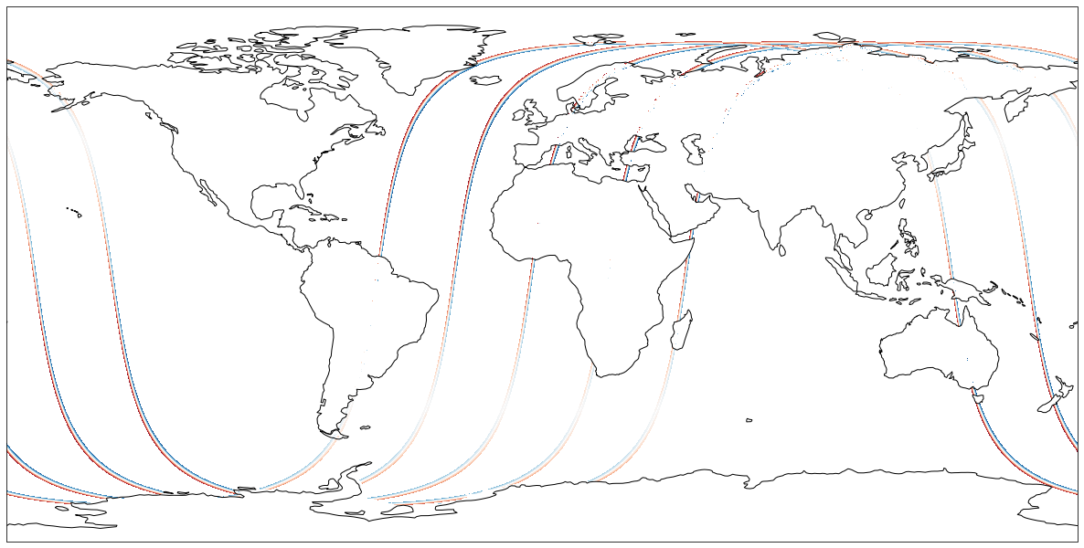
A final word…
Accessing data completely from S3 and in memory are affected by various things.
- The format of the data - archive formats like NetCDF, GEOTIFF, HDF vs cloud optimized data structures (Zarr, kerchunk, COG). Cloud formats are made for accessing only the pieces of data of interest needed at the time of the request (e.g. a subset, timestep, etc).
- The internal structure of the data. Tools like xarray make a lot of assumptions about how to open and read a file. Sometimes the internals don’t fit the xarray ‘mould’ and we need to continue to work with data providers and software providers to make these two sides work together. Level 2 data (non-gridded), specifically, suffers from some of the assumptions made.