import glob
import os
import requests
import s3fs
import fiona
import netCDF4 as nc
import h5netcdf
import xarray as xr
import pandas as pd
import geopandas as gpd
import numpy as np
import matplotlib.pyplot as plt
import hvplot.xarray
import earthaccess
from earthaccess import Auth, DataCollections, DataGranules, StoreFor an updated notebook using the latest data, see this notebook in the PO.DAAC Cookbook
SWOT Hydrology Dataset Exploration in the Cloud
Accessing and Visualizing SWOT Datasets
Requirement:
This tutorial can only be run in an AWS cloud instance running in us-west-2: NASA Earthdata Cloud data in S3 can be directly accessed via earthaccess python library; this access is limited to requests made within the US West (Oregon) (code: us-west-2) AWS region.
Learning Objectives:
- Access SWOT HR data prodcuts (archived in NASA Earthdata Cloud) within the AWS cloud, without downloading to local machine
- Visualize accessed data for a quick check
SWOT Level 2 KaRIn High Rate Version 1.1 (where available) Datasets:
River Vector Shapefile - SWOT_L2_HR_RIVERSP_1.1
Lake Vector Shapefile - SWOT_L2_HR_LAKESP_1.1
Water Mask Pixel Cloud NetCDF - SWOT_L2_HR_PIXC_1.1
Water Mask Pixel Cloud Vector Attribute NetCDF - SWOT_L2_HR_PIXCVec_1.1
Raster NetCDF - SWOT_L2_HR_Raster_1.1
Single Look Complex Data product - SWOT_L1B_HR_SLC_1.1
Notebook Author: Cassie Nickles, NASA PO.DAAC (Aug 2023) || Other Contributors: Zoe Walschots (PO.DAAC Summer Intern 2023), Catalina Taglialatela (NASA PO.DAAC), Luis Lopez (NASA NSIDC DAAC)
Last updated: 4 Dec 2023
Libraries Needed
Earthdata Login
An Earthdata Login account is required to access data, as well as discover restricted data, from the NASA Earthdata system. Thus, to access NASA data, you need Earthdata Login. If you don’t already have one, please visit https://urs.earthdata.nasa.gov to register and manage your Earthdata Login account. This account is free to create and only takes a moment to set up. We use earthaccess to authenticate your login credentials below.
auth = earthaccess.login()Single File Access
1. River Vector Shapefiles
The s3 access link can be found using earthaccess data search. Since this collection consists of Reach and Node files, we need to extract only the granule for the Reach file. We do this by filtering for the ‘Reach’ title in the data link.
Alternatively, Earthdata Search (see tutorial) can be used to search in a map graphic user interface.
For additional tips on spatial searching of SWOT HR L2 data, see also PO.DAAC Cookbook - SWOT Chapter tips section.
Search for the data of interest
# Retrieves granule from the day we want, in this case by passing to `earthdata.search_data` function the data collection shortname, temporal bounds, and for restricted data one must specify the search count
river_results = earthaccess.search_data(short_name = 'SWOT_L2_HR_RIVERSP_1.1',
temporal = ('2023-04-08 00:00:00', '2023-04-22 23:59:59'),
granule_name = '*Reach*_024_NA*') # here we filter by Reach files (not node), pass #24 and continent code=NA for North America
# granule_name = '*Reach*_013_NA*') # here we filter by Reach files (not node), pass #13 and continent code=NAGranules found: 15Set up an s3fs session for Direct Cloud Access
s3fs sessions are used for authenticated access to s3 bucket and allows for typical file-system style operations. Below we create session by passing in the data access information.
fs_s3 = earthaccess.get_s3fs_session(results=river_results)Create Fiona session to work with zip and embedded shapefiles in the AWS Cloud
The native format for this data is a .zip file, and we want the .shp file within the .zip file, so we will create a Fiona AWS session using the credentials from setting up the s3fs session above to access the shapefiles within the zip files. If we don’t do this, the alternative would be to download the data to the cloud environment (e.g. EC2 instance, user S3 bucket) and extract the .zip file there.
fiona_session=fiona.session.AWSSession(
aws_access_key_id=fs_s3.storage_options["key"],
aws_secret_access_key=fs_s3.storage_options["secret"],
aws_session_token=fs_s3.storage_options["token"]
)# Get the link for the first zip file
river_link = earthaccess.results.DataGranule.data_links(river_results[0], access='direct')[0]
# We use the zip+ prefix so fiona knows that we are operating on a zip file
river_shp_url = f"zip+{river_link}"
with fiona.Env(session=fiona_session):
SWOT_HR_shp1 = gpd.read_file(river_shp_url)
#view the attribute table
SWOT_HR_shp1 | reach_id | time | time_tai | time_str | p_lat | p_lon | river_name | wse | wse_u | wse_r_u | ... | p_wid_var | p_n_nodes | p_dist_out | p_length | p_maf | p_dam_id | p_n_ch_max | p_n_ch_mod | p_low_slp | geometry | |
|---|---|---|---|---|---|---|---|---|---|---|---|---|---|---|---|---|---|---|---|---|---|
| 0 | 71185400013 | 7.342856e+08 | 7.342856e+08 | 2023-04-08T16:12:43Z | 55.405348 | -106.628388 | no_data | 3.864838e+02 | 1.139410e+00 | 1.135850e+00 | ... | 7863771.149 | 48 | 61917.017 | 9521.873154 | -1.000000e+12 | 0 | 10 | 2 | 0 | LINESTRING (-106.60903 55.44509, -106.60930 55... |
| 1 | 71185400021 | 7.342856e+08 | 7.342856e+08 | 2023-04-08T16:12:43Z | 55.452342 | -106.601114 | no_data | -1.000000e+12 | -1.000000e+12 | -1.000000e+12 | ... | 0.000 | 10 | 53346.297 | 1902.305299 | -1.000000e+12 | 0 | 5 | 1 | 0 | LINESTRING (-106.59293 55.45986, -106.59320 55... |
| 2 | 71185400033 | -1.000000e+12 | -1.000000e+12 | no_data | 55.632220 | -106.451323 | no_data | -1.000000e+12 | -1.000000e+12 | -1.000000e+12 | ... | 758315.173 | 14 | 28676.430 | 2858.149671 | -1.000000e+12 | 0 | 7 | 2 | 0 | LINESTRING (-106.47121 55.62881, -106.47073 55... |
| 3 | 71185400041 | 7.342856e+08 | 7.342856e+08 | 2023-04-08T16:12:43Z | 55.361687 | -106.646694 | no_data | 3.861999e+02 | 9.139000e-02 | 1.588000e-02 | ... | 0.000 | 5 | 62976.523 | 1059.505878 | -1.000000e+12 | 0 | 5 | 1 | 0 | LINESTRING (-106.64608 55.36668, -106.64607 55... |
| 4 | 71185400053 | 7.342856e+08 | 7.342856e+08 | 2023-04-08T16:12:43Z | 55.350062 | -106.647210 | no_data | 3.861795e+02 | 1.022600e-01 | 4.855000e-02 | ... | 3214.190 | 8 | 64492.945 | 1516.422084 | -1.000000e+12 | 0 | 1 | 1 | 0 | LINESTRING (-106.64728 55.35669, -106.64736 55... |
| ... | ... | ... | ... | ... | ... | ... | ... | ... | ... | ... | ... | ... | ... | ... | ... | ... | ... | ... | ... | ... | ... |
| 594 | 75211000291 | -1.000000e+12 | -1.000000e+12 | no_data | 26.100287 | -98.270345 | Rio Bravo | -1.000000e+12 | -1.000000e+12 | -1.000000e+12 | ... | 123.027 | 53 | 238333.030 | 10660.888100 | -1.000000e+12 | 0 | 1 | 1 | 0 | LINESTRING (-98.25015 26.07251, -98.25039 26.0... |
| 595 | 75211000301 | -1.000000e+12 | -1.000000e+12 | no_data | 26.115209 | -98.305631 | Rio Grande | -1.000000e+12 | -1.000000e+12 | -1.000000e+12 | ... | 242.204 | 53 | 248976.010 | 10642.980241 | -1.000000e+12 | 0 | 1 | 1 | 0 | LINESTRING (-98.27467 26.11517, -98.27497 26.1... |
| 596 | 75211000683 | 7.342861e+08 | 7.342861e+08 | 2023-04-08T16:21:20Z | 25.955223 | -97.159176 | Rio Grande | 2.871000e-01 | 9.005000e-02 | 3.080000e-03 | ... | 436.214 | 18 | 9238.006 | 3611.160551 | -1.000000e+12 | 0 | 1 | 1 | 0 | LINESTRING (-97.14980 25.95092, -97.15011 25.9... |
| 597 | 75211000691 | 7.342861e+08 | 7.342861e+08 | 2023-04-08T16:21:20Z | 25.957129 | -97.209134 | Rio Grande | 3.374000e-01 | 9.102000e-02 | 1.360000e-02 | ... | 348.855 | 53 | 19926.935 | 10688.929343 | -1.000000e+12 | 0 | 1 | 1 | 0 | LINESTRING (-97.16943 25.96060, -97.16972 25.9... |
| 598 | 75211000701 | 7.342861e+08 | 7.342861e+08 | 2023-04-08T16:21:20Z | 25.945001 | -97.279869 | Rio Grande | 4.375000e-01 | 9.212000e-02 | 1.965000e-02 | ... | 203.786 | 53 | 30608.499 | 10681.563344 | -1.000000e+12 | 0 | 1 | 1 | 0 | LINESTRING (-97.25170 25.94769, -97.25200 25.9... |
599 rows × 127 columns
Quickly plot the SWOT river data
# Simple plot
fig, ax = plt.subplots(figsize=(7,5))
SWOT_HR_shp1.plot(ax=ax, color='black')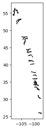
# # Another way to plot geopandas dataframes is with `explore`, which also plots a basemap
SWOT_HR_shp1.explore()Make this Notebook Trusted to load map: File -> Trust Notebook
2. Lake Vector Shapefiles
The lake vector shapefiles can be accessed in the same way as the river shapefiles above.
For additional tips on spatial searching of SWOT HR L2 data, see also PO.DAAC Cookbook - SWOT Chapter tips section.
Search for data of interest
lake_results = earthaccess.search_data(short_name = 'SWOT_L2_HR_LAKESP_1.1',
temporal = ('2023-04-08 00:00:00', '2023-04-22 23:59:59'),
granule_name = '*Obs*_024_NA*')
# granule_name = '*Obs*_013_NA*') # here we filter by files with 'Obs' in the name (This collection has three options: Obs, Unassigned, and Prior), pass #13 and continent code=NAGranules found: 15Set up an s3fs session for Direct Cloud Access
s3fs sessions are used for authenticated access to s3 bucket and allows for typical file-system style operations. Below we create session by passing in the data access information.
fs_s3 = earthaccess.get_s3fs_session(results=lake_results)Create Fiona session to work with zip and embedded shapefiles in the AWS Cloud
The native format for this data is a .zip file, and we want the .shp file within the .zip file, so we will create a Fiona AWS session using the credentials from setting up the s3fs session above to access the shapefiles within the zip files. If we don’t do this, the alternative would be to download the data to the cloud environment (e.g. EC2 instance, user S3 bucket) and extract the .zip file there.
fiona_session=fiona.session.AWSSession(
aws_access_key_id=fs_s3.storage_options["key"],
aws_secret_access_key=fs_s3.storage_options["secret"],
aws_session_token=fs_s3.storage_options["token"]
)# Get the link for the first zip file
lake_link = earthaccess.results.DataGranule.data_links(lake_results[0], access='direct')[0]
# We use the zip+ prefix so fiona knows that we are operating on a zip file
lake_shp_url = f"zip+{lake_link}"
with fiona.Env(session=fiona_session):
SWOT_HR_shp2 = gpd.read_file(lake_shp_url)
#view the attribute table
SWOT_HR_shp2| obs_id | lake_id | overlap | n_overlap | reach_id | time | time_tai | time_str | wse | wse_u | ... | load_tidef | load_tideg | pole_tide | dry_trop_c | wet_trop_c | iono_c | xovr_cal_c | lake_name | p_res_id | geometry | |
|---|---|---|---|---|---|---|---|---|---|---|---|---|---|---|---|---|---|---|---|---|---|
| 0 | 711056R000000 | 7110058862 | 43 | 1 | no_data | 7.342856e+08 | 7.342856e+08 | 2023-04-08T16:12:42Z | 456.591 | 0.068 | ... | 0.012544 | 0.011979 | -0.001644 | -2.171307 | -0.096968 | -0.004681 | -1.000000e+12 | no_data | -99999999 | POLYGON ((-108.10263 55.82828, -108.10271 55.8... |
| 1 | 711056R000006 | 7110057883;7110044502 | 32;0 | 2 | 71185900011;71185900023;71185900031;7118590004... | 7.342856e+08 | 7.342856e+08 | 2023-04-08T16:12:47Z | 420.100 | 0.043 | ... | 0.012521 | 0.011962 | -0.001645 | -2.179560 | -0.095098 | -0.004694 | -1.000000e+12 | ILE-A-LA-CROSSE | -99999999 | MULTIPOLYGON (((-108.04803 55.51018, -108.0481... |
| 2 | 711056R000002 | 7110044512;7110045352 | 93;2 | 2 | no_data | 7.342856e+08 | 7.342856e+08 | 2023-04-08T16:12:43Z | 423.307 | 0.130 | ... | 0.012743 | 0.012195 | -0.001671 | -2.177715 | -0.099736 | -0.004680 | -1.000000e+12 | PETER POND;NISKA LAKE | -99999999 | MULTIPOLYGON (((-108.63716 55.67995, -108.6372... |
| 3 | 711056R000003 | 7110044502 | 0 | 1 | no_data | 7.342856e+08 | 7.342856e+08 | 2023-04-08T16:12:42Z | 421.265 | 0.718 | ... | 0.012595 | 0.012031 | -0.001651 | -2.178498 | -0.098505 | -0.004681 | -1.000000e+12 | FROBISHER LAKE;NIPAWIN BAY;PETER POND LAKE;CHU... | -99999999 | MULTIPOLYGON (((-108.22462 55.77025, -108.2251... |
| 4 | 711056R001623 | 7110061392 | 70 | 1 | no_data | 7.342856e+08 | 7.342856e+08 | 2023-04-08T16:12:52Z | 433.682 | 0.159 | ... | 0.012518 | 0.011977 | -0.001648 | -2.176805 | -0.093354 | -0.004701 | -1.000000e+12 | AMYOT LAKE | -99999999 | MULTIPOLYGON (((-107.87588 55.21497, -107.8759... |
| ... | ... | ... | ... | ... | ... | ... | ... | ... | ... | ... | ... | ... | ... | ... | ... | ... | ... | ... | ... | ... | ... |
| 5084 | 753111R000533 | 7530074612 | 33 | 1 | no_data | 7.342861e+08 | 7.342861e+08 | 2023-04-08T16:21:48Z | 1.204 | 0.151 | ... | 0.003597 | 0.004175 | -0.001930 | -2.332590 | -0.261529 | -0.010383 | -1.000000e+12 | no_data | -99999999 | MULTIPOLYGON (((-97.73272 25.04506, -97.73275 ... |
| 5085 | 753111R000813 | 7530075482 | 9 | 1 | no_data | 7.342861e+08 | 7.342861e+08 | 2023-04-08T16:21:48Z | 0.851 | 0.166 | ... | 0.003638 | 0.004185 | -0.001905 | -2.332652 | -0.261308 | -0.010385 | -1.000000e+12 | no_data | -99999999 | POLYGON ((-97.74014 25.04083, -97.74030 25.041... |
| 5086 | 753111R000849 | 7530072312 | 82 | 1 | no_data | 7.342861e+08 | 7.342861e+08 | 2023-04-08T16:21:48Z | 0.507 | 0.058 | ... | 0.003659 | 0.004194 | -0.001900 | -2.332774 | -0.261139 | -0.010385 | -1.000000e+12 | no_data | -99999999 | POLYGON ((-97.75064 25.04090, -97.75067 25.041... |
| 5087 | 753111R000883 | 7530075482 | 66 | 1 | no_data | 7.342861e+08 | 7.342861e+08 | 2023-04-08T16:21:48Z | 0.577 | 0.027 | ... | 0.003676 | 0.004200 | -0.001788 | -2.332951 | -0.261053 | -0.010387 | -1.000000e+12 | no_data | -99999999 | MULTIPOLYGON (((-97.76046 25.03127, -97.76049 ... |
| 5088 | 753111R000978 | 7530075052 | 50 | 1 | no_data | 7.342861e+08 | 7.342861e+08 | 2023-04-08T16:21:48Z | 3.190 | 0.062 | ... | 0.003768 | 0.004261 | -0.001394 | -2.332381 | -0.260291 | -0.010385 | -1.000000e+12 | no_data | -99999999 | MULTIPOLYGON (((-97.79919 25.02889, -97.79933 ... |
5089 rows × 36 columns
Quickly plot the SWOT lakes data
fig, ax = plt.subplots(figsize=(7,5))
SWOT_HR_shp2.plot(ax=ax, color='black')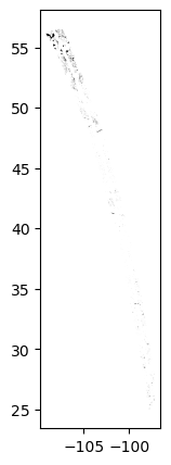
# # Another way to plot geopandas dataframes is with `explore`, which also plots a basemap
# SWOT_HR_shp2.explore()# # [Optional] Diving a bit deeper, plotting riversP and lakeSP overlaid on same map
# m = SWOT_HR_shp1.explore() #define the riverSP map
# SWOT_HR_shp2.explore(m=m, color="orange") #plot the riverSP with the lakesSP data, where lakes are in orangeAccessing the remaining files is different than the shp files above. We do not need to read the shapefiles within a zip file using something like Fiona session (or to download and unzip in the cloud) because the following SWOT HR collections are stored in netCDF files in the cloud. For the rest of the products, we will open via xarray, not geopandas.
3. Water Mask Pixel Cloud NetCDF
Search for data collection and time of interest
For additional tips on spatial searching of SWOT HR L2 data, see also PO.DAAC Cookbook - SWOT Chapter tips section.
pixc_results = earthaccess.search_data(short_name = 'SWOT_L2_HR_PIXC_1.1',
temporal = ('2023-04-22 00:00:00', '2023-04-22 23:59:59'),
granule_name = '*_498_024_101L*')
# granule_name = '*_498_013_*') # here we filter by cycle=498 and pass=013 Granules found: 1Set up an s3fs session for Direct Cloud Access
s3fs sessions are used for authenticated access to s3 bucket and allows for typical file-system style operations. Below we create session by passing in the data access information.
fs_s3 = earthaccess.get_s3fs_session(results=pixc_results)
# get link for file 1
pixc_link = earthaccess.results.DataGranule.data_links(pixc_results[0], access='direct')[0]
s3_file_obj3 = fs_s3.open(pixc_link, mode='rb')Open data using xarray
The pixel cloud netCDF files are formatted with three groups titled, “pixel cloud”, “tvp”, or “noise” (more detail here). In order to access the coordinates and variables within the file, a group must be specified when calling xarray open_dataset.
ds_PIXC = xr.open_dataset(s3_file_obj3, group = 'pixel_cloud', engine='h5netcdf')
ds_PIXC<xarray.Dataset>
Dimensions: (points: 6842667, complex_depth: 2,
num_pixc_lines: 3249)
Coordinates:
latitude (points) float64 ...
longitude (points) float64 ...
Dimensions without coordinates: points, complex_depth, num_pixc_lines
Data variables: (12/57)
azimuth_index (points) float64 ...
range_index (points) float64 ...
interferogram (points, complex_depth) float32 ...
power_plus_y (points) float32 ...
power_minus_y (points) float32 ...
coherent_power (points) float32 ...
... ...
interferogram_qual (points) float64 ...
classification_qual (points) float64 ...
geolocation_qual (points) float64 ...
sig0_qual (points) float64 ...
pixc_line_qual (num_pixc_lines) float64 ...
pixc_line_to_tvp (num_pixc_lines) float32 ...
Attributes:
description: cloud of geolocated interferogram pixels
interferogram_size_azimuth: 3249
interferogram_size_range: 4758
looks_to_efflooks: 1.5368636877472777
num_azimuth_looks: 7.0
azimuth_offset: 8Simple plot of the results
# This could take a few minutes to plot
plt.scatter(x=ds_PIXC.longitude, y=ds_PIXC.latitude, c=ds_PIXC.height)
plt.colorbar().set_label('Height (m)')
# plt.scatter(x=ds_PIXC.longitude, y=ds_PIXC.latitude, c=ds_PIXC.classification)
# plt.colorbar().set_label('Classification')4. Water Mask Pixel Cloud Vector Attribute NetCDF
Search for data of interest
pixcvec_results = earthaccess.search_data(short_name = 'SWOT_L2_HR_PIXCVEC_1.1',
temporal = ('2023-04-08 00:00:00', '2023-04-22 23:59:59'),
granule_name = '*_498_024_101L*')
# granule_name = '*_498_013_*') # here we filter by cycle=498 and pass=013 Granules found: 1Set up an s3fs session for Direct Cloud Access
s3fs sessions are used for authenticated access to s3 bucket and allows for typical file-system style operations. Below we create session by passing in the data access information.
fs_s3 = earthaccess.get_s3fs_session(results=pixcvec_results)
# get link for file 0
pixcvec_link = earthaccess.results.DataGranule.data_links(pixcvec_results[0], access='direct')[0]
s3_file_obj4 = fs_s3.open(pixcvec_link, mode='rb')Open data using xarray
ds_PIXCVEC = xr.open_dataset(s3_file_obj4, decode_cf=False, engine='h5netcdf')
ds_PIXCVEC<xarray.Dataset>
Dimensions: (points: 6842667, nchar_reach_id: 11,
nchar_node_id: 14, nchar_lake_id: 10,
nchar_obs_id: 13)
Dimensions without coordinates: points, nchar_reach_id, nchar_node_id,
nchar_lake_id, nchar_obs_id
Data variables:
azimuth_index (points) int32 ...
range_index (points) int32 ...
latitude_vectorproc (points) float64 ...
longitude_vectorproc (points) float64 ...
height_vectorproc (points) float32 ...
reach_id (points, nchar_reach_id) |S1 ...
node_id (points, nchar_node_id) |S1 ...
lake_id (points, nchar_lake_id) |S1 ...
obs_id (points, nchar_obs_id) |S1 ...
ice_clim_f (points) int8 ...
ice_dyn_f (points) int8 ...
Attributes: (12/45)
Conventions: CF-1.7
title: Level 2 KaRIn high rate pixel cloud vect...
short_name: L2_HR_PIXCVec
institution: JPL
source: Level 1B KaRIn High Rate Single Look Com...
history: 2023-10-03T00:34:10.665297Z: Creation
... ...
xref_prior_river_db_file:
xref_prior_lake_db_file: SWOT_LakeDatabase_Cal_024_20000101T00000...
xref_reforbittrack_files: SWOT_RefOrbitTrackTileBoundary_Cal_20000...
xref_param_l2_hr_laketile_file: SWOT_Param_L2_HR_LakeTile_20000101T00000...
ellipsoid_semi_major_axis: 6378137.0
ellipsoid_flattening: 0.0033528106647474805Simple plot
pixcvec_htvals = ds_PIXCVEC.height_vectorproc.compute()
pixcvec_latvals = ds_PIXCVEC.latitude_vectorproc.compute()
pixcvec_lonvals = ds_PIXCVEC.longitude_vectorproc.compute()
#Before plotting, we set all fill values to nan so that the graph shows up better spatially
pixcvec_htvals[pixcvec_htvals > 15000] = np.nan
pixcvec_latvals[pixcvec_latvals < 1] = np.nan
pixcvec_lonvals[pixcvec_lonvals > -1] = np.nanplt.scatter(x=pixcvec_lonvals, y=pixcvec_latvals, c=pixcvec_htvals)
plt.colorbar().set_label('Height (m)')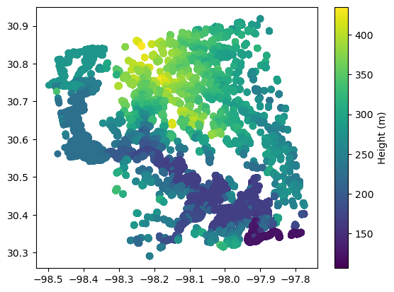
5. Raster NetCDF
Search for data of interest
For additional tips on spatial searching of SWOT HR L2 data, see also PO.DAAC Cookbook - SWOT Chapter tips section.
#Say we know the exact cycle, pass & scene. We can search for one data granule!
raster_results = earthaccess.search_data(short_name = 'SWOT_L2_HR_Raster_1.1',
temporal = ('2023-04-01 00:00:00', '2023-04-22 23:59:59'),
granule_name = '*100m*_498_024_051F*')
# granule_name = '*100m*_498_013_130F*') # here we filter by files with '100m' in the name (This collection has two resolution options: 100m & 250m), cycle=498, pass=013, scene = 130F Granules found: 1Set up an s3fs session for Direct Cloud Access
s3fs sessions are used for authenticated access to s3 bucket and allows for typical file-system style operations. Below we create session by passing in the data access information.
fs_s3 = earthaccess.get_s3fs_session(results=raster_results)
# get link for file
raster_link = earthaccess.results.DataGranule.data_links(raster_results[0], access='direct')[0]
s3_file_obj5 = fs_s3.open(raster_link, mode='rb')Open data with xarray
ds_raster = xr.open_dataset(s3_file_obj5, engine='h5netcdf')
ds_raster<xarray.Dataset>
Dimensions: (x: 1505, y: 1505)
Coordinates:
* x (x) float64 4.855e+05 4.856e+05 ... 6.359e+05
* y (y) float64 3.272e+06 3.272e+06 ... 3.422e+06
Data variables: (12/39)
crs object ...
longitude (y, x) float64 ...
latitude (y, x) float64 ...
wse (y, x) float32 ...
wse_qual (y, x) float32 ...
wse_qual_bitwise (y, x) float64 ...
... ...
load_tide_fes (y, x) float32 ...
load_tide_got (y, x) float32 ...
pole_tide (y, x) float32 ...
model_dry_tropo_cor (y, x) float32 ...
model_wet_tropo_cor (y, x) float32 ...
iono_cor_gim_ka (y, x) float32 ...
Attributes: (12/49)
Conventions: CF-1.7
title: Level 2 KaRIn High Rate Raster Data Product
source: Ka-band radar interferometer
history: 2023-10-04T10:18:05Z : Creation
platform: SWOT
reference_document: JPL D-56416 - Revision B - October 24, 2022
... ...
x_max: 635900.0
y_min: 3271900.0
y_max: 3422300.0
institution: JPL
references: V1.0
product_version: 01Quick interactive plot with hvplot
ds_raster.wse.hvplot.image(y='y', x='x')