For an updated notebook using the latest data, see this notebook in the PO.DAAC Cookbook

SWOT Hydrology Science Application Tutorial on the Cloud

Retrieving SWOT attributes (WSE, width, slope) and plotting a longitudinal profile along a river or over a basin

Requirement

This tutorial can only be run in an AWS cloud instance running in us-west-2: NASA Earthdata Cloud data in S3 can be directly accessed via earthaccess python library; this access is limited to requests made within the US West (Oregon) (code: us-west-2) AWS region.

Earthdata Login

An Earthdata Login account is required to access data, as well as discover restricted data, from the NASA Earthdata system. Thus, to access NASA data, you need Earthdata Login. Please visit https://urs.earthdata.nasa.gov to register and manage your Earthdata Login account. This account is free to create and only takes a moment to set up.

This code runs using SWOT Level 2 Data Products (Version 1.1).

Notebook Authors: Arnaud Cerbelaud, Jeffrey Wade, NASA Jet Propulsion Laboratory - California Institute of Technology (Jan 2024)

Learning Objectives

Retrieve SWOT hydrological attributes on river reaches within the AWS cloud (Cal/Val data). Query reaches by:
- River name
- Spatial bounding box
- Downstream tracing from reach id (e.g. headwater to outlet) for river longitudinal profiles
- Upstream tracing from reach id (e.g. outlet to full river network) for watershed analysis
Plot a time series of WSE, width, slope data on the filtered data
Visualize an interactive map of WSE, width, slope data on the filtered data

Last updated: 2 Feb 2024

Import Packages

import glob
import os
import requests
import s3fs
import fiona
import netCDF4 as nc
import h5netcdf
import xarray as xr
import pandas as pd
import geopandas as gpd
import numpy as np
import matplotlib.pyplot as plt
import hvplot.xarray
import earthaccess
from earthaccess import Auth, DataCollections, DataGranules, Store
from pathlib import Path
import zipfile

Authenticate

Authenticate your Earthdata Login (EDL) information using the earthaccess python package as follows:

earthaccess.login() # Login with your EDL credentials if asked

Enter your Earthdata Login username:  cerbelaud
Enter your Earthdata password:  ········

<earthaccess.auth.Auth at 0x7f114ba7bd30>

1. Retrieve SWOT hydrological attributes on river reaches within the AWS cloud (Cal/Val data)

What data should we download?

Optional step: Get the .kmz file of SWOT passes/swaths (Version 1.1) and import it into Google Earth for visualization
Determine which pass number corresponds to the river/basin you want to look at! #### Search for multiple days of data

# Enter pass number
pass_number    = "009"   # e.g. 009 for Connecticut in NA, 003 for Rhine in EU
# Enter continent code
continent_code = "NA"     # e.g. "AF", "NA", "EU", "SI", "AS", "AU", "SA", "AR", "GR"

# Retrieves granule from the day we want, in this case by passing to `earthdata.search_data` function the data collection shortname and temporal bounds
river_results = earthaccess.search_data(short_name = 'SWOT_L2_HR_RIVERSP_1.1', 
                                        temporal = ('2023-04-08 00:00:00', '2023-04-12 23:59:59'),
                                        granule_name = "*Reach*_" + pass_number + "_" + continent_code + "*")

# Create fiona session to read data
fs_s3 = earthaccess.get_s3fs_session(results=river_results)
fiona_session=fiona.session.AWSSession(
        aws_access_key_id=fs_s3.storage_options["key"],
        aws_secret_access_key=fs_s3.storage_options["secret"],
        aws_session_token=fs_s3.storage_options["token"]
    )

Granules found: 5

Unzip selected files in Fiona session

# Initialize list of shapefiles containing all dates
SWOT_HR_shps = []

# Loop through queried granules to stack all acquisition dates
for j in range(len(river_results)):
    
    # Get the link for each zip file
    river_link = earthaccess.results.DataGranule.data_links(river_results[j], access='direct')[0]
    
    # We use the zip+ prefix so fiona knows that we are operating on a zip file
    river_shp_url = f"zip+{river_link}"
    
    # Read shapefile
    with fiona.Env(session=fiona_session):
        SWOT_HR_shps.append(gpd.read_file(river_shp_url))

Aggregate unzipped files into dataframe

# Combine granules from all acquisition dates into one dataframe
SWOT_HR_df = gpd.GeoDataFrame(pd.concat(SWOT_HR_shps, ignore_index=True))

# Sort dataframe by reach_id and time
SWOT_HR_df = SWOT_HR_df.sort_values(['reach_id', 'time'])

SWOT_HR_df

	reach_id	time	time_tai	time_str	p_lat	p_lon	river_name	wse	wse_u	wse_r_u	...	p_wid_var	p_n_nodes	p_dist_out	p_length	p_maf	p_dam_id	p_n_ch_max	p_n_ch_mod	p_low_slp	geometry
1958	72270400231	-1.000000e+12	-1.000000e+12	no_data	56.794630	-66.461122	no_data	-1.000000e+12	-1.000000e+12	-1.000000e+12	...	1618.079	53	230079.472	10630.774958	-1.000000e+12	0	1	1	0	LINESTRING (-66.48682 56.83442, -66.48645 56.8...
2641	72270400231	-1.000000e+12	-1.000000e+12	no_data	56.794630	-66.461122	no_data	-1.000000e+12	-1.000000e+12	-1.000000e+12	...	1618.079	53	230079.472	10630.774958	-1.000000e+12	0	1	1	0	LINESTRING (-66.48682 56.83442, -66.48645 56.8...
1959	72270400241	-1.000000e+12	-1.000000e+12	no_data	56.744361	-66.341905	no_data	-1.000000e+12	-1.000000e+12	-1.000000e+12	...	4831.128	53	240728.430	10648.958289	-1.000000e+12	0	2	1	0	LINESTRING (-66.41602 56.75969, -66.41553 56.7...
2642	72270400241	-1.000000e+12	-1.000000e+12	no_data	56.744361	-66.341905	no_data	-1.000000e+12	-1.000000e+12	-1.000000e+12	...	4831.128	53	240728.430	10648.958289	-1.000000e+12	0	2	1	0	LINESTRING (-66.41602 56.75969, -66.41553 56.7...
1960	72270400251	7.344991e+08	7.344991e+08	2023-04-11T03:31:02Z	56.676087	-66.219811	no_data	2.855340e+02	1.008930e+00	1.004910e+00	...	412.975	58	252286.769	11558.339052	-1.000000e+12	0	2	1	0	LINESTRING (-66.27812 56.71437, -66.27775 56.7...
...	...	...	...	...	...	...	...	...	...	...	...	...	...	...	...	...	...	...	...	...	...
615	73130000061	-1.000000e+12	-1.000000e+12	no_data	41.424945	-73.230960	Housatonic River	-1.000000e+12	-1.000000e+12	-1.000000e+12	...	10469.706	82	47161.191	16303.793847	-1.000000e+12	0	2	1	0	LINESTRING (-73.17436 41.38295, -73.17465 41.3...
1283	73130000061	-1.000000e+12	-1.000000e+12	no_data	41.424945	-73.230960	Housatonic River	-1.000000e+12	-1.000000e+12	-1.000000e+12	...	10469.706	82	47161.191	16303.793847	-1.000000e+12	0	2	1	0	LINESTRING (-73.17436 41.38295, -73.17465 41.3...
1957	73130000061	-1.000000e+12	-1.000000e+12	no_data	41.424945	-73.230960	Housatonic River	-1.000000e+12	-1.000000e+12	-1.000000e+12	...	10469.706	82	47161.191	16303.793847	-1.000000e+12	0	2	1	0	LINESTRING (-73.17436 41.38295, -73.17465 41.3...
2640	73130000061	-1.000000e+12	-1.000000e+12	no_data	41.424945	-73.230960	Housatonic River	-1.000000e+12	-1.000000e+12	-1.000000e+12	...	10469.706	82	47161.191	16303.793847	-1.000000e+12	0	2	1	0	LINESTRING (-73.17436 41.38295, -73.17465 41.3...
3312	73130000061	-1.000000e+12	-1.000000e+12	no_data	41.424945	-73.230960	Housatonic River	-1.000000e+12	-1.000000e+12	-1.000000e+12	...	10469.706	82	47161.191	16303.793847	-1.000000e+12	0	2	1	0	LINESTRING (-73.17436 41.38295, -73.17465 41.3...

3313 rows × 127 columns

Exploring the dataset

What acquisition dates and rivers do our downloaded files cover?

print('Available dates are:')
print(np.unique([i[:10] for i in SWOT_HR_df['time_str']]))
print('Available rivers are:')
print(np.unique([i for i in SWOT_HR_df['river_name']]))

Available dates are:
['2023-04-08' '2023-04-09' '2023-04-10' '2023-04-11' '2023-04-12'
 'no_data']
Available rivers are:
['Allagash River' 'Androscoggin River' 'Big Black River' 'Canal de fuite'
 'Carrabassett River' 'Concord River' 'Concord River; Sudbury River'
 'Connecticut River' 'Connecticut River; Westfield River'
 'Connecticut River; White River' 'Dead River'
 'Dead River (Kennebec River)' 'Deerfield River' 'Farmington River'
 'Housatonic River' 'Ikarut River' 'Kennebec River' 'Komaktorvik River'
 'Magalloway River' 'Merrimack River' 'Moose River'
 'North Branch Penobscot River' 'Passumsic River' 'Pemigewasset River'
 'Penobscot River West Branch' 'Quinebaug River' 'Saco River'
 'Saguenay River' 'Saint Francis River' 'Saint John River'
 'Saint Lawrence River' 'Sandy River' 'Shetucket River' 'Sudbury River'
 'Thames River' 'West River' 'White River' 'no_data']

Filter dataframe by river name of interest and plot selected reaches:

Note: Some rivers have multiple names, hence using the contains function

# Enter river name
river = "Connecticut River"  # e.g. "Rhine", "Connecticut River"

## Filter dataframe
SWOT_HR_df_river = SWOT_HR_df[(SWOT_HR_df.river_name.str.contains(river))]

# Plot geopandas dataframe with 'explore' by reach id
SWOT_HR_df_river[['reach_id','river_name','geometry']].explore('reach_id', style_kwds=dict(weight=6))

Make this Notebook Trusted to load map: File -> Trust Notebook

Filter dataframe by latitude/longitude of interest:

lat_start = {"Connecticut River": 41.5,
             "Rhine": 47.5
            }
lat_end   = {"Connecticut River": 45,
             "Rhine": 51
            }
lon_start = {"Connecticut River": -74,
             "Rhine": 7
            }
lon_end   = {"Connecticut River": -71,
             "Rhine": 10
            }

## Filter dataframe
SWOT_HR_df_box = SWOT_HR_df[(SWOT_HR_df.p_lat > lat_start[river]) & (SWOT_HR_df.p_lat < lat_end[river]) & (SWOT_HR_df.p_lon > lon_start[river]) & (SWOT_HR_df.p_lon < lon_end[river])]

# Plot geopandas dataframe with 'explore' by river name
SWOT_HR_df_box[['reach_id','river_name','geometry']].explore('river_name', style_kwds=dict(weight=6))

Make this Notebook Trusted to load map: File -> Trust Notebook

2. River longitudinal profile: trace reaches downstream of given starting reach using `rch_id_dn` field

WARNING: This works as long as the data is exhaustive (no missing SWORD reaches)

First, let’s set up a dictionary relating all reaches in the dataset to their downstream neighbor

Note: rch_dn_dict[rch_id] gives a list of all the reaches directly downstream from rch_id

# Format rch_id_dn for dictionary. Rch_id_dn allows for multiple downstream reaches to be stored
# Also removes spaces in attribute field
rch_id_dn = [[x.strip() for x in SWOT_HR_df.rch_id_dn[j].split(',')] for j in range(0,len(SWOT_HR_df.rch_id_dn))]

# Filter upstream reach ids to remove 'no_data'
rch_id_dn_filter = [[x for x in dn_id if x.isnumeric()] for dn_id in rch_id_dn]

# Create lookup dictionary for river network topology: Downstream
rch_dn_dict = {SWOT_HR_df.reach_id[i]: rch_id_dn_filter[i] for i in range(len(SWOT_HR_df))}

Then, starting from a given reach, let’s trace all connected downstream reaches

# Enter reach_id from which we will trace downstream    (e.g. headwaters of the Connecticut River)
rch_dn_st = {"Connecticut River": '73120000691',
             "Rhine": '23267000651'
            }

# Initialize list to store downstream reaches, including starting reach
rch_dn_list = [rch_dn_st[river]]
# Retrieve first downstream id of starting reach and add to list
rch_dn_next = rch_dn_dict[rch_dn_st[river]][0]

# Trace next downstream reach until we hit the outlet (or here the last reach on file)
while len(rch_dn_next) != 0:
    # Add reach to list if value exists
    if len(rch_dn_next) != 0:
        rch_dn_list.append(rch_dn_next)
    # Recursively retrieve first downstream id of next reach
    # Catch error if reach isn't in downloaded data
    try:
        rch_dn_next = rch_dn_dict[rch_dn_next][0]
    except:
        break

Finally, we filtered our downloaded data by the traced reaches to create a plot

# Filter downloaded data by downstream traced reaches
SWOT_dn_trace = SWOT_HR_df[SWOT_HR_df.reach_id.isin(rch_dn_list)]

# Remove reaches from rch_dn_list that are not present in SWOT data
rch_dn_list = [rch for rch in rch_dn_list if rch in SWOT_HR_df.reach_id.values]

SWOT_dn_trace[['reach_id','river_name','geometry']].explore('river_name', style_kwds=dict(weight=6))

Make this Notebook Trusted to load map: File -> Trust Notebook

3. Watershed analysis: trace reaches upstream of starting reach using `rch_id_up` field

WARNING: This works as long as the data is exhaustive (no missing SWORD reaches)

First, let’s set up a dictionary relating all reaches in the dataset to their upstream neighbor

Note: rch_up_dict[rch_id] gives a list of all the reaches directly upstream from rch_id

# Format rch_id_up for dictionary. Rch_id_up allows for multiple upstream reaches to be stored
# Also removes spaces in attribute field
rch_id_up = [[x.strip() for x in SWOT_HR_df.rch_id_up[j].split(',')] for j in range(0,len(SWOT_HR_df.rch_id_up))]

# Filter upstream reach ids to remove 'no_data'
rch_id_up_fil = [[x for x in ups_id if x.isnumeric()] for ups_id in rch_id_up]

# Create lookup dictionary for river network topology: Upstream
rch_up_dict = {SWOT_HR_df.reach_id[i]: rch_id_up_fil[i] for i in range(len(SWOT_HR_df))}

Then, starting from a given reach, let’s trace all connected upstream reaches

This adds a bit of complexity, as we need to keep track of multiple branches upstream of the starting reach.

# Enter reach_id from which we will trace upstream    (e.g. outlet of the Connecticut River)
rch_up_st = {"Connecticut River": '73120000013',
             "Rhine": '23265000051'
            }

# Initialize list to store traced upstream reaches, including starting reach
rch_up_list = [rch_up_st[river]]
# Retrieve ids of reaches upstream of starting reach and add to list
rch_up_next = rch_up_dict[rch_up_st[river]]
# For upstream tracing, we need to set a list of next upstream ids to start while loop
rch_next_id = rch_up_next

# Loop until no more reaches to trace
while len(rch_next_id) != 0:
    # Initialize list to store next upstream ids
    rch_next_id = []
    # Loop through next upstream ids for given reach
    for rch_up_sel in rch_up_next:
        # Get values of existing upstream ids of rch_up_next reaches
        # If reach isn't in SWOT data (usually ghost reaches), continue to next reach
        try:
            rch_next_id = rch_next_id + rch_up_dict[rch_up_sel]
        except:
            continue
        # Append id to list
        rch_up_list.append(rch_up_sel)
    # If reaches exist, add to list for next cycle of tracing
    if len(rch_next_id) != 0:
        rch_up_next = rch_next_id

Finally, we filtered our downloaded data by the traced reaches to create a plot

# Filter downloaded data by upstream traced reaches
SWOT_up_trace = SWOT_HR_df[SWOT_HR_df.reach_id.isin(rch_up_list)]

# Remove reaches from rch_up_list that are not present in SWOT data
rch_up_list = [rch for rch in rch_up_list if rch in SWOT_HR_df.reach_id.values]

SWOT_up_trace[['reach_id','river_name','geometry']].explore('river_name', style_kwds=dict(weight=6))

Make this Notebook Trusted to load map: File -> Trust Notebook

4. Visualize and plot a time series of WSE/width/slope longitudinal profiles

Let’s create a time series dataframe from the downstream filtered database

# Retrieve all possible acquisition dates (keeping only YYYY-MM-DD)
dates = np.unique([i[:10] for i in [x for x in SWOT_HR_df['time_str'] if x!='no_data']])

# Create a new database for time series analysis with unique reach_ids
SWOT_dn_trace_time = SWOT_dn_trace.set_index('reach_id').groupby(level=0) \
                                  .apply(lambda df: df.reset_index(drop=True)) \
                                  .unstack().sort_index(axis=1, level=1)

SWOT_dn_trace_time.columns = ['{}_{}'.format(x[0],dates[x[1]]) for x in SWOT_dn_trace_time.columns]

Plot a longitudinal profile for selected SWOT variable

# Explore variables you could choose to plot
for var in ["wse","slope","width","len"]:
    print(SWOT_dn_trace.columns[SWOT_dn_trace.columns.str.contains(var)])

Index(['wse', 'wse_u', 'wse_r_u', 'wse_c', 'wse_c_u', 'area_wse', 'p_wse',
       'p_wse_var'],
      dtype='object')
Index(['slope', 'slope_u', 'slope_r_u', 'slope2', 'slope2_u', 'slope2_r_u'], dtype='object')
Index(['width', 'width_u', 'width_c', 'width_c_u', 'p_width'], dtype='object')
Index(['p_length'], dtype='object')

# Enter variable of interest for plotting
varstr = "wse"

# Find cumulative length on the longitudinal profile
length_list    = np.nan_to_num([SWOT_dn_trace.p_length[SWOT_dn_trace.reach_id == rch].mean()/1000 for rch in rch_dn_list])
cumlength_list = np.cumsum(length_list)

## Plot a longitudinal profile from the downstream tracing database

## Plot a longitudinal profile from the downstream tracing database
plt.figure(figsize=(12,8))
for t in dates:
    
    # Store the quantity of interest (wse, width etc.) at time t
    value = SWOT_dn_trace_time.loc[rch_dn_list,varstr+'_'+t]
    
    # Remove set negative values (bad observations) to NaN and forward fill NaNs
    value[value < 0] = np.nan
    value = value.ffill()
    
    # Plot the data
    plt.plot(cumlength_list, value, label = varstr+'_'+t)
    
plt.xlabel('Downstream Distance (km)')
plt.ylabel(varstr)
plt.legend()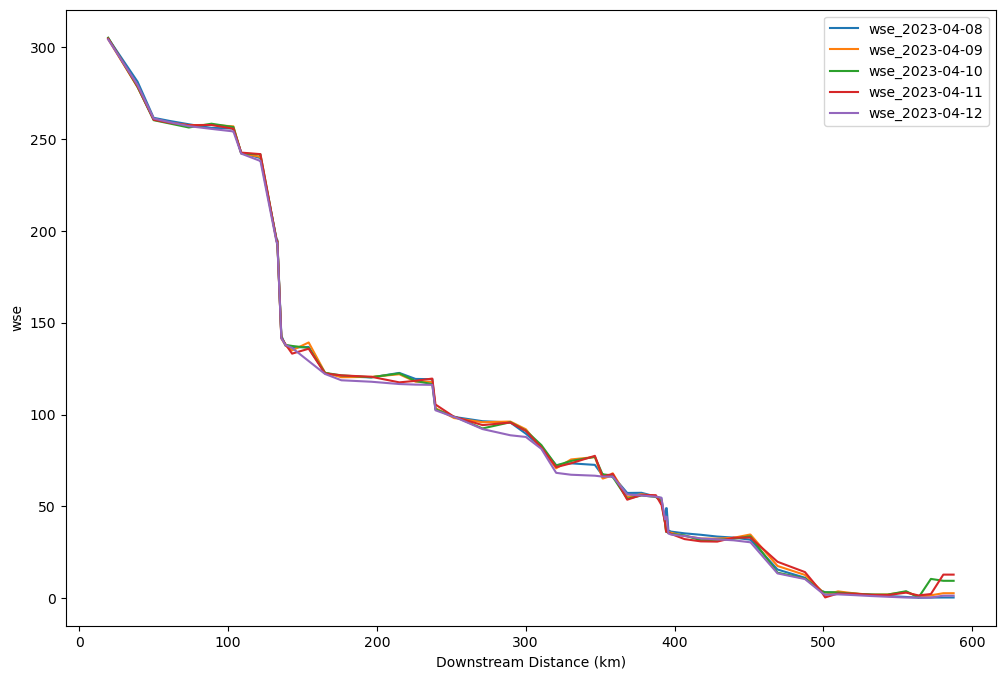

Map the longitudinal profile of selected SWOT variable

# Choose a date
date = dates[0]

#Set one column as the active geometry in the new database
SWOT_dn_trace_time = SWOT_dn_trace_time.set_geometry("geometry_"+date)

#Set cleaner colorbar bounds for better visualization
vmin = np.percentile([i for i in SWOT_dn_trace_time[varstr+'_'+date] if i>0],5)
vmax = np.percentile([i for i in SWOT_dn_trace_time[varstr+'_'+date] if i>0],95)

# Interactive map
SWOT_dn_trace_time.explore(varstr+'_'+date,
                           vmin = vmin,
                           vmax = vmax,
                           cmap = "Blues", #"Blues",
                           control_scale = True,
                           tooltip = varstr+'_'+dates[0],  # show "varstr+'_'+dates[0]" value in tooltip (on hover)
                           popup = True,  # show all values in popup (on click)
                           #tiles = "CartoDB positron",  # use "CartoDB positron" tiles
                           style_kwds=dict(weight=10)
                          )

Make this Notebook Trusted to load map: File -> Trust Notebook

Supplemental

We can also map the upstream traced database

SWOT_up_trace_time = SWOT_up_trace.set_index('reach_id').groupby(level=0) \
                                  .apply(lambda df: df.reset_index(drop=True)) \
                                  .unstack().sort_index(axis=1, level=1)

SWOT_up_trace_time.columns = ['{}_{}'.format(x[0],dates[x[1]]) for x in SWOT_up_trace_time.columns]

SWOT_up_trace_time = SWOT_up_trace_time.set_geometry("geometry_"+date)

#Set cleaner colorbar bounds for better visualization
vmin = np.percentile([i for i in SWOT_up_trace_time[varstr+'_'+date] if i>0],5)
vmax = np.percentile([i for i in SWOT_up_trace_time[varstr+'_'+date] if i>0],95)

# Interactive map
SWOT_up_trace_time.explore(varstr+'_'+date,
                           vmin = vmin,
                           vmax = vmax,
                           cmap = "Blues", #"Blues",
                           control_scale = True,
                           tooltip = varstr+'_'+dates[0],  # show "varstr+'_'+dates[0]" value in tooltip (on hover)
                           popup = True,  # show all values in popup (on click)
                           tiles = "CartoDB positron",  # use "CartoDB positron" tiles
                           style_kwds=dict(weight=5)
                          )

Make this Notebook Trusted to load map: File -> Trust Notebook

How to filter out raster data to reveal water bodies?

Now you will also need the tile number (in addition to the pass number). You can find it on the .kmz file

# Enter tile number
tile_number = "116F"

# Retrieve granules from all days to find the cycle corresponding to the desired date
raster_results = earthaccess.search_data(short_name = 'SWOT_L2_HR_Raster_1.1', 
                                         temporal = ('2023-04-01 00:00:00', '2023-04-22 23:59:59'), 
                                         granule_name = "*100m*_" + pass_number + "_" + tile_number + "*")
# here we filter by files with '100m' in the name, pass=009, scene = 116F (tile = 232L) for Connecticut
                                                 # pass=003, scene = 120F (tile = 239R) for the Rhine

Granules found: 15

Display details of downloaded files

print([i for i in raster_results])

[Collection: {'Version': '1.1', 'ShortName': 'SWOT_L2_HR_Raster_1.1'}
Spatial coverage: {'HorizontalSpatialDomain': {'Orbit': {'StartLatitude': -77.66, 'EndLatitude': 77.66, 'AscendingCrossing': -80.4, 'StartDirection': 'A', 'EndDirection': 'A'}, 'Track': {'Cycle': 484, 'Passes': [{'Pass': 9, 'Tiles': ['230L', '231L', '232L', '233L', '230R', '231R', '232R', '233R']}]}}}
Temporal coverage: {'RangeDateTime': {'EndingDateTime': '2023-04-08T03:55:38.288Z', 'BeginningDateTime': '2023-04-08T03:55:18.398Z'}}
Size(MB): 70.40732002258301
Data: ['https://archive.swot.podaac.earthdata.nasa.gov/podaac-swot-ops-cumulus-protected/SWOT_L2_HR_Raster_1.1/SWOT_L2_HR_Raster_100m_UTM19T_N_x_x_x_484_009_116F_20230408T035517_20230408T035538_PIB0_01.nc'], Collection: {'Version': '1.1', 'ShortName': 'SWOT_L2_HR_Raster_1.1'}
Spatial coverage: {'HorizontalSpatialDomain': {'Orbit': {'StartLatitude': -77.66, 'EndLatitude': 77.66, 'AscendingCrossing': -80.4, 'StartDirection': 'A', 'EndDirection': 'A'}, 'Track': {'Cycle': 485, 'Passes': [{'Pass': 9, 'Tiles': ['230L', '231L', '232L', '233L', '230R', '231R', '232R', '233R']}]}}}
Temporal coverage: {'RangeDateTime': {'EndingDateTime': '2023-04-09T03:46:16.448Z', 'BeginningDateTime': '2023-04-09T03:45:56.558Z'}}
Size(MB): 68.41873073577881
Data: ['https://archive.swot.podaac.earthdata.nasa.gov/podaac-swot-ops-cumulus-protected/SWOT_L2_HR_Raster_1.1/SWOT_L2_HR_Raster_100m_UTM19T_N_x_x_x_485_009_116F_20230409T034556_20230409T034616_PIB0_01.nc'], Collection: {'Version': '1.1', 'ShortName': 'SWOT_L2_HR_Raster_1.1'}
Spatial coverage: {'HorizontalSpatialDomain': {'Orbit': {'StartLatitude': -77.66, 'EndLatitude': 77.66, 'AscendingCrossing': -80.4, 'StartDirection': 'A', 'EndDirection': 'A'}, 'Track': {'Cycle': 486, 'Passes': [{'Pass': 9, 'Tiles': ['230L', '231L', '232L', '233L', '230R', '231R', '232R', '233R']}]}}}
Temporal coverage: {'RangeDateTime': {'EndingDateTime': '2023-04-10T03:36:54.573Z', 'BeginningDateTime': '2023-04-10T03:36:34.684Z'}}
Size(MB): 68.47044467926025
Data: ['https://archive.swot.podaac.earthdata.nasa.gov/podaac-swot-ops-cumulus-protected/SWOT_L2_HR_Raster_1.1/SWOT_L2_HR_Raster_100m_UTM19T_N_x_x_x_486_009_116F_20230410T033634_20230410T033655_PIB0_01.nc'], Collection: {'Version': '1.1', 'ShortName': 'SWOT_L2_HR_Raster_1.1'}
Spatial coverage: {'HorizontalSpatialDomain': {'Orbit': {'StartLatitude': -77.66, 'EndLatitude': 77.66, 'AscendingCrossing': -80.4, 'StartDirection': 'A', 'EndDirection': 'A'}, 'Track': {'Cycle': 487, 'Passes': [{'Pass': 9, 'Tiles': ['230L', '231L', '232L', '233L', '230R', '231R', '232R', '233R']}]}}}
Temporal coverage: {'RangeDateTime': {'EndingDateTime': '2023-04-11T03:27:32.662Z', 'BeginningDateTime': '2023-04-11T03:27:12.772Z'}}
Size(MB): 69.02541446685791
Data: ['https://archive.swot.podaac.earthdata.nasa.gov/podaac-swot-ops-cumulus-protected/SWOT_L2_HR_Raster_1.1/SWOT_L2_HR_Raster_100m_UTM19T_N_x_x_x_487_009_116F_20230411T032712_20230411T032733_PIB0_01.nc'], Collection: {'Version': '1.1', 'ShortName': 'SWOT_L2_HR_Raster_1.1'}
Spatial coverage: {'HorizontalSpatialDomain': {'Orbit': {'StartLatitude': -77.66, 'EndLatitude': 77.66, 'AscendingCrossing': -80.4, 'StartDirection': 'A', 'EndDirection': 'A'}, 'Track': {'Cycle': 488, 'Passes': [{'Pass': 9, 'Tiles': ['230L', '231L', '232L', '233L', '230R', '231R', '232R', '233R']}]}}}
Temporal coverage: {'RangeDateTime': {'EndingDateTime': '2023-04-12T03:18:10.720Z', 'BeginningDateTime': '2023-04-12T03:17:50.831Z'}}
Size(MB): 67.56003761291504
Data: ['https://archive.swot.podaac.earthdata.nasa.gov/podaac-swot-ops-cumulus-protected/SWOT_L2_HR_Raster_1.1/SWOT_L2_HR_Raster_100m_UTM19T_N_x_x_x_488_009_116F_20230412T031750_20230412T031811_PIB0_01.nc'], Collection: {'Version': '1.1', 'ShortName': 'SWOT_L2_HR_Raster_1.1'}
Spatial coverage: {'HorizontalSpatialDomain': {'Orbit': {'StartLatitude': -77.66, 'EndLatitude': 77.66, 'AscendingCrossing': -80.4, 'StartDirection': 'A', 'EndDirection': 'A'}, 'Track': {'Cycle': 489, 'Passes': [{'Pass': 9, 'Tiles': ['230L', '231L', '232L', '233L', '230R', '231R', '232R', '233R']}]}}}
Temporal coverage: {'RangeDateTime': {'EndingDateTime': '2023-04-13T03:08:48.751Z', 'BeginningDateTime': '2023-04-13T03:08:28.862Z'}}
Size(MB): 68.72685241699219
Data: ['https://archive.swot.podaac.earthdata.nasa.gov/podaac-swot-ops-cumulus-protected/SWOT_L2_HR_Raster_1.1/SWOT_L2_HR_Raster_100m_UTM19T_N_x_x_x_489_009_116F_20230413T030828_20230413T030849_PIB0_01.nc'], Collection: {'Version': '1.1', 'ShortName': 'SWOT_L2_HR_Raster_1.1'}
Spatial coverage: {'HorizontalSpatialDomain': {'Orbit': {'StartLatitude': -77.66, 'EndLatitude': 77.66, 'AscendingCrossing': -80.4, 'StartDirection': 'A', 'EndDirection': 'A'}, 'Track': {'Cycle': 490, 'Passes': [{'Pass': 9, 'Tiles': ['230L', '231L', '232L', '233L', '230R', '231R', '232R', '233R']}]}}}
Temporal coverage: {'RangeDateTime': {'EndingDateTime': '2023-04-14T02:59:26.753Z', 'BeginningDateTime': '2023-04-14T02:59:06.866Z'}}
Size(MB): 66.47898387908936
Data: ['https://archive.swot.podaac.earthdata.nasa.gov/podaac-swot-ops-cumulus-protected/SWOT_L2_HR_Raster_1.1/SWOT_L2_HR_Raster_100m_UTM19T_N_x_x_x_490_009_116F_20230414T025906_20230414T025927_PIB0_01.nc'], Collection: {'Version': '1.1', 'ShortName': 'SWOT_L2_HR_Raster_1.1'}
Spatial coverage: {'HorizontalSpatialDomain': {'Orbit': {'StartLatitude': -77.66, 'EndLatitude': 77.66, 'AscendingCrossing': -80.41, 'StartDirection': 'A', 'EndDirection': 'A'}, 'Track': {'Cycle': 491, 'Passes': [{'Pass': 9, 'Tiles': ['230L', '231L', '232L', '233L', '230R', '231R', '232R', '233R']}]}}}
Temporal coverage: {'RangeDateTime': {'EndingDateTime': '2023-04-15T02:50:04.726Z', 'BeginningDateTime': '2023-04-15T02:49:44.836Z'}}
Size(MB): 67.29588985443115
Data: ['https://archive.swot.podaac.earthdata.nasa.gov/podaac-swot-ops-cumulus-protected/SWOT_L2_HR_Raster_1.1/SWOT_L2_HR_Raster_100m_UTM19T_N_x_x_x_491_009_116F_20230415T024944_20230415T025005_PIB0_01.nc'], Collection: {'Version': '1.1', 'ShortName': 'SWOT_L2_HR_Raster_1.1'}
Spatial coverage: {'HorizontalSpatialDomain': {'Orbit': {'StartLatitude': -77.66, 'EndLatitude': 77.66, 'AscendingCrossing': -80.41, 'StartDirection': 'A', 'EndDirection': 'A'}, 'Track': {'Cycle': 492, 'Passes': [{'Pass': 9, 'Tiles': ['230L', '231L', '232L', '233L', '230R', '231R', '232R', '233R']}]}}}
Temporal coverage: {'RangeDateTime': {'EndingDateTime': '2023-04-16T02:40:43.207Z', 'BeginningDateTime': '2023-04-16T02:40:22.244Z'}}
Size(MB): 0.933258056640625
Data: ['https://archive.swot.podaac.earthdata.nasa.gov/podaac-swot-ops-cumulus-protected/SWOT_L2_HR_Raster_1.1/SWOT_L2_HR_Raster_100m_UTM19T_N_x_x_x_492_009_116F_20230416T024022_20230416T024043_PIB0_01.nc'], Collection: {'Version': '1.1', 'ShortName': 'SWOT_L2_HR_Raster_1.1'}
Spatial coverage: {'HorizontalSpatialDomain': {'Orbit': {'StartLatitude': -77.66, 'EndLatitude': 77.66, 'AscendingCrossing': -80.41, 'StartDirection': 'A', 'EndDirection': 'A'}, 'Track': {'Cycle': 493, 'Passes': [{'Pass': 9, 'Tiles': ['230L', '231L', '232L', '233L', '230R', '231R', '232R', '233R']}]}}}
Temporal coverage: {'RangeDateTime': {'EndingDateTime': '2023-04-17T02:31:21.112Z', 'BeginningDateTime': '2023-04-17T02:31:00.151Z'}}
Size(MB): 0.9332094192504883
Data: ['https://archive.swot.podaac.earthdata.nasa.gov/podaac-swot-ops-cumulus-protected/SWOT_L2_HR_Raster_1.1/SWOT_L2_HR_Raster_100m_UTM19T_N_x_x_x_493_009_116F_20230417T023100_20230417T023121_PIB0_01.nc'], Collection: {'Version': '1.1', 'ShortName': 'SWOT_L2_HR_Raster_1.1'}
Spatial coverage: {'HorizontalSpatialDomain': {'Orbit': {'StartLatitude': -77.66, 'EndLatitude': 77.66, 'AscendingCrossing': -80.41, 'StartDirection': 'A', 'EndDirection': 'A'}, 'Track': {'Cycle': 494, 'Passes': [{'Pass': 9, 'Tiles': ['230L', '231L', '232L', '233L', '230R', '231R', '232R', '233R']}]}}}
Temporal coverage: {'RangeDateTime': {'EndingDateTime': '2023-04-18T02:21:58.990Z', 'BeginningDateTime': '2023-04-18T02:21:38.024Z'}}
Size(MB): 0.9332304000854492
Data: ['https://archive.swot.podaac.earthdata.nasa.gov/podaac-swot-ops-cumulus-protected/SWOT_L2_HR_Raster_1.1/SWOT_L2_HR_Raster_100m_UTM19T_N_x_x_x_494_009_116F_20230418T022138_20230418T022158_PIB0_01.nc'], Collection: {'Version': '1.1', 'ShortName': 'SWOT_L2_HR_Raster_1.1'}
Spatial coverage: {'HorizontalSpatialDomain': {'Orbit': {'StartLatitude': -77.66, 'EndLatitude': 77.66, 'AscendingCrossing': -80.41, 'StartDirection': 'A', 'EndDirection': 'A'}, 'Track': {'Cycle': 495, 'Passes': [{'Pass': 9, 'Tiles': ['230L', '231L', '232L', '233L', '230R', '231R', '232R', '233R']}]}}}
Temporal coverage: {'RangeDateTime': {'EndingDateTime': '2023-04-19T02:12:36.279Z', 'BeginningDateTime': '2023-04-19T02:12:16.394Z'}}
Size(MB): 63.773990631103516
Data: ['https://archive.swot.podaac.earthdata.nasa.gov/podaac-swot-ops-cumulus-protected/SWOT_L2_HR_Raster_1.1/SWOT_L2_HR_Raster_100m_UTM19T_N_x_x_x_495_009_116F_20230419T021215_20230419T021236_PIB0_01.nc'], Collection: {'Version': '1.1', 'ShortName': 'SWOT_L2_HR_Raster_1.1'}
Spatial coverage: {'HorizontalSpatialDomain': {'Orbit': {'StartLatitude': -77.66, 'EndLatitude': 77.66, 'AscendingCrossing': -80.41, 'StartDirection': 'A', 'EndDirection': 'A'}, 'Track': {'Cycle': 496, 'Passes': [{'Pass': 9, 'Tiles': ['230L', '231L', '232L', '233L', '230R', '231R', '232R', '233R']}]}}}
Temporal coverage: {'RangeDateTime': {'EndingDateTime': '2023-04-20T02:03:14.075Z', 'BeginningDateTime': '2023-04-20T02:02:54.187Z'}}
Size(MB): 62.185853004455566
Data: ['https://archive.swot.podaac.earthdata.nasa.gov/podaac-swot-ops-cumulus-protected/SWOT_L2_HR_Raster_1.1/SWOT_L2_HR_Raster_100m_UTM19T_N_x_x_x_496_009_116F_20230420T020253_20230420T020314_PIB0_01.nc'], Collection: {'Version': '1.1', 'ShortName': 'SWOT_L2_HR_Raster_1.1'}
Spatial coverage: {'HorizontalSpatialDomain': {'Orbit': {'StartLatitude': -77.66, 'EndLatitude': 77.66, 'AscendingCrossing': -80.41, 'StartDirection': 'A', 'EndDirection': 'A'}, 'Track': {'Cycle': 497, 'Passes': [{'Pass': 9, 'Tiles': ['230L', '231L', '232L', '233L', '230R', '231R', '232R', '233R']}]}}}
Temporal coverage: {'RangeDateTime': {'EndingDateTime': '2023-04-21T01:53:51.831Z', 'BeginningDateTime': '2023-04-21T01:53:31.942Z'}}
Size(MB): 61.36593437194824
Data: ['https://archive.swot.podaac.earthdata.nasa.gov/podaac-swot-ops-cumulus-protected/SWOT_L2_HR_Raster_1.1/SWOT_L2_HR_Raster_100m_UTM19T_N_x_x_x_497_009_116F_20230421T015331_20230421T015352_PIB0_01.nc'], Collection: {'Version': '1.1', 'ShortName': 'SWOT_L2_HR_Raster_1.1'}
Spatial coverage: {'HorizontalSpatialDomain': {'Orbit': {'StartLatitude': -77.66, 'EndLatitude': 77.66, 'AscendingCrossing': -80.41, 'StartDirection': 'A', 'EndDirection': 'A'}, 'Track': {'Cycle': 498, 'Passes': [{'Pass': 9, 'Tiles': ['230L', '231L', '232L', '233L', '230R', '231R', '232R', '233R']}]}}}
Temporal coverage: {'RangeDateTime': {'EndingDateTime': '2023-04-22T01:44:29.616Z', 'BeginningDateTime': '2023-04-22T01:44:09.731Z'}}
Size(MB): 61.341376304626465
Data: ['https://archive.swot.podaac.earthdata.nasa.gov/podaac-swot-ops-cumulus-protected/SWOT_L2_HR_Raster_1.1/SWOT_L2_HR_Raster_100m_UTM19T_N_x_x_x_498_009_116F_20230422T014409_20230422T014430_PIB0_01.nc']]

Select a single file for visualization

# Let's look at cycle 485, on the second day of calval
# Enter cycle
cycle = "485"

raster_results = earthaccess.search_data(short_name = 'SWOT_L2_HR_Raster_1.1', 
                                         temporal = ('2023-04-01 00:00:00', '2023-04-22 23:59:59'), 
                                         granule_name = "*100m*" + cycle + "_" + pass_number + "_" + tile_number + "*")

# here we filter by files with '100m' in the name, cycle=484, pass=009, scene = 116F for Connecticut
                                                 # cycle=485, pass=003, scene = 120F for the Rhine

Granules found: 1

Open file using fiona AWS session and read file using xarray

fs_s3 = earthaccess.get_s3fs_session(results=raster_results)

# get link for file and open it
raster_link = earthaccess.results.DataGranule.data_links(raster_results[0], access='direct')[0]
s3_file_obj5 = fs_s3.open(raster_link, mode='rb')

# Open data with xarray
ds_raster = xr.open_dataset(s3_file_obj5, engine='h5netcdf')

Plot raster data using custom filters to improve image quality

# Plot the data with a filter on water_frac > x, or sig0>50
ds_raster.wse.where(ds_raster.water_frac > 0.5).hvplot.image(y='y', x='x').opts(cmap='Blues', clim=(vmin,vmax), width=1000, height=750)

SWOT Hydrology Science Application Tutorial on the Cloud

Retrieving SWOT attributes (WSE, width, slope) and plotting a longitudinal profile along a river or over a basin

Requirement

Earthdata Login

Learning Objectives

Import Packages

Authenticate

1. Retrieve SWOT hydrological attributes on river reaches within the AWS cloud (Cal/Val data)

What data should we download?

Unzip selected files in Fiona session

Aggregate unzipped files into dataframe

Exploring the dataset

What acquisition dates and rivers do our downloaded files cover?

Filter dataframe by river name of interest and plot selected reaches:

Filter dataframe by latitude/longitude of interest:

2. River longitudinal profile: trace reaches downstream of given starting reach using rch_id_dn field

First, let’s set up a dictionary relating all reaches in the dataset to their downstream neighbor

Then, starting from a given reach, let’s trace all connected downstream reaches

Finally, we filtered our downloaded data by the traced reaches to create a plot

3. Watershed analysis: trace reaches upstream of starting reach using rch_id_up field

First, let’s set up a dictionary relating all reaches in the dataset to their upstream neighbor

Then, starting from a given reach, let’s trace all connected upstream reaches

Finally, we filtered our downloaded data by the traced reaches to create a plot

4. Visualize and plot a time series of WSE/width/slope longitudinal profiles

Let’s create a time series dataframe from the downstream filtered database

Plot a longitudinal profile for selected SWOT variable

Map the longitudinal profile of selected SWOT variable

Supplemental

We can also map the upstream traced database

How to filter out raster data to reveal water bodies?

Display details of downloaded files

Select a single file for visualization

Open file using fiona AWS session and read file using xarray

Plot raster data using custom filters to improve image quality

2. River longitudinal profile: trace reaches downstream of given starting reach using `rch_id_dn` field

3. Watershed analysis: trace reaches upstream of starting reach using `rch_id_up` field