import icechunk
import xarray as xr
import earthaccessFrom the PO.DAAC Cookbook, to access the GitHub version of the notebook, follow this link.
Example of Opening an Icechunk Store In-Cloud
Author: Dean Henze, PO.DAAC
This notebook demonstrates opening a virtual dataset (VDS) stored as an Icechunk store (note this technology is currently experimental, although it is gaining momentum). For a general overview of VDS’s see the Using Virutal Datasets chapter on the PO.DAAC Cookbook.
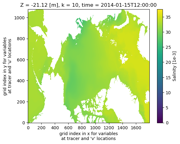
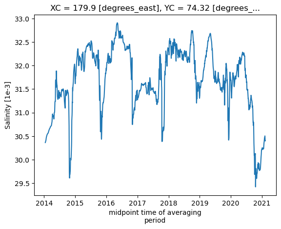
The example dataset(s) used here are from the SASSIE ECCO project (the User Guide has a project overview). The ECCO model (Estimating the Circulation and Climate of the Ocean) was run over the arctic region over a seven year period in support of the SASSIE field experiment (Salinity and Stratification at the Sea Ice Edge). The SASSIE ECCO data are traditionally archived and available in netCDF format - one file per day(month) for the daily-mean(monthly-snapshot) datasets. The model output variables (totalling ~50 TBs) are large enough that they are spread out over 18 different netCDF datasets for the daily-means, and over 3 different datasets for the monthly-snapshots. One novel functionality of VDS’s being tested here is the ability to combine the data across e.g. the 18 daily-mean datasets so users can interact with the data as if all variables were contained in a single dataset. Computing performance is TBD.
The AWS S3 paths to the SASSIE ECCO icechunk stores are
Daily averages:
s3://podaac-ops-cumulus-public/virtual_collections/SASSIE_ECCO_V1R1/SASSIE_ECCO_L4_DAILY_V1R1_virtual_s3.icechunk/
Monthly snapshots:
s3://podaac-ops-cumulus-public/virtual_collections/SASSIE_ECCO_V1R1/SASSIE_ECCO_L4_SNAPSHOT_V1R1_virtual_s3.icechunk/
Requirements and Python environment
Earthdata login account: An Earthdata Login account is required to access data from the NASA Earthdata system. Please visit https://urs.earthdata.nasa.gov to register and manage your Earthdata Login account.
Compute environment: This notebook is meant to be run in the cloud (AWS instance running in us-west-2).
The minimal working installation for Python 3.13 environment is
earthaccess==0.16.0
icechunk==1.1.19
xarray==2025.6.1
zarr==3.1.1
matplotlib
jupyterlab
Note that the icechunk=1.1.19 dependency is important! Do not use a more recent version.
1. Define a function to access the icechunk store
This function does not need any modification. It defines some access keywords and a mapper to the VDS. The mapper will contain all the required access credentials and can be passed directly to xarray. In the future this step will likely be built into to earthaccess but for now we must define it in the notebook. The only inputs to the function are:
- Your EDS credentials
- The link to the VDS reference file (in the header of this notebook and in the next section).
def open_readonly_icechunkstore_s3(
                           s3path_store, creds_store, creds_data_chunks,
                           bucket_data_chunks = "s3://podaac-ops-cumulus-protected/"):
    """
    Opens and returns an icechunk store with read-only capabilities.

    Inputs
    ------
    s3path_store: str or path
        AWS S3 path to the icechunk store, e.g. "s3://podaac-ops-cumulus-public/virtual_collections/...".
    creds_store: dict
        Credentials to access the icechunk store (e.g. EDL creds for NASA Earthdata). Expected
        dictionary keys are "accessKeyId", "secretAccessKey", and "sessionToken".
    creds_data_chunks: dict
        Credentials to access the science data that the icechunk store points to (e.g. EDL creds
        for NASA Earthdata). Expected dictionary keys are "accessKeyId", "secretAccessKey",
        and "sessionToken".
    bucket_data_chunks: str
        Name of bucket containing the science data that the icechunk store points to. E.g. for
        PO.DAAC data this might be "s3://podaac-ops-cumulus-protected/". Note you need
        the "s3://" prefix.
    """


    # 1. Create the raw static credentials object for virtual chunks
    virtualchunk_static_creds = icechunk.s3_static_credentials(
        access_key_id = creds_data_chunks["accessKeyId"],
        secret_access_key = creds_data_chunks["secretAccessKey"],
        session_token = creds_data_chunks["sessionToken"]
    )
    auth_map = icechunk.containers_credentials({
        bucket_data_chunks: virtualchunk_static_creds
    })

    # 2. Config for the store / metadata repository
    s3path_split = s3path_store.split("/")
    bucket_store = "/".join(s3path_split[2:3])
    prefix_store = "/".join(s3path_split[3:])

    storage = icechunk.s3_storage(
        bucket = bucket_store,
        prefix = prefix_store,
        access_key_id = creds_store['accessKeyId'],
        secret_access_key = creds_store['secretAccessKey'],
        session_token = creds_store['sessionToken']
    )

    # 3. Open the repository, passing the compiled auth_map!
    repo = icechunk.Repository.open(
        storage,
        authorize_virtual_chunk_access=auth_map
    )

    # 4. Return the store
    session = repo.readonly_session("main")
    return session.store
2. Access store and open data with Xarray
Steps are to:
- Login to NASA EDL.
- Use the above function to get the icechunk store mapper.
- Pass the mapper into Xarray to open the dataset.
- Perform some sample computations
Enter your Earthdata Login username:  deanh808
Enter your Earthdata password:  ········
The AWS S3 paths to the SASSIE ECCO icechunk stores are
Daily averages:
s3://podaac-ops-cumulus-public/virtual_collections/SASSIE_ECCO_V1R1/SASSIE_ECCO_L4_DAILY_V1R1_virtual_s3.icechunk/
Monthly snapshots:
s3://podaac-ops-cumulus-public/virtual_collections/SASSIE_ECCO_V1R1/SASSIE_ECCO_L4_SNAPSHOT_V1R1_virtual_s3.icechunk/
## 2. Get the icechunk store mapper  ----------------------------------------------------------------------------------
s3path_store = "s3://podaac-ops-cumulus-public/virtual_collections/SASSIE_ECCO_V1R1/SASSIE_ECCO_L4_DAILY_V1R1_virtual_s3.icechunk/"
store = open_readonly_icechunkstore_s3(
    s3path_store,
    ea_creds, ea_creds,
    bucket_data_chunks = "s3://podaac-ops-cumulus-protected/"
)/opt/coiled/env/lib/python3.14/site-packages/zarr/codecs/numcodecs/_codecs.py:141: ZarrUserWarning: Numcodecs codecs are not in the Zarr version 3 specification and may not be supported by other zarr implementations.
super().__init__(**codec_config)CPU times: user 828 ms, sys: 163 ms, total: 991 ms
Wall time: 1.58 s<xarray.Dataset> Size: 46TB
Dimensions: (time: 2581, k_l: 90, j: 1080, i: 1800, i_g: 1800, j_g: 1080,
k: 90, k_u: 90, nb: 4, k_p1: 91, nv: 2)
Coordinates: (12/23)
XC (j, i) float32 8MB dask.array<chunksize=(1080, 1800), meta=np.ndarray>
XC_bnds (j, i, nb) float32 31MB dask.array<chunksize=(1080, 1800, 4), meta=np.ndarray>
YC (j, i) float32 8MB dask.array<chunksize=(1080, 1800), meta=np.ndarray>
XU (j, i_g) float32 8MB dask.array<chunksize=(1080, 1800), meta=np.ndarray>
YC_bnds (j, i, nb) float32 31MB dask.array<chunksize=(1080, 1800, 4), meta=np.ndarray>
YU (j, i_g) float32 8MB dask.array<chunksize=(1080, 1800), meta=np.ndarray>
... ...
* j_g (j_g) int32 4kB 0 1 2 3 4 5 6 ... 1074 1075 1076 1077 1078 1079
* k_p1 (k_p1) int32 364B 0 1 2 3 4 5 6 7 8 ... 83 84 85 86 87 88 89 90
* k_l (k_l) int32 360B 0 1 2 3 4 5 6 7 8 ... 81 82 83 84 85 86 87 88 89
time_bnds (time, nv) datetime64[ns] 41kB dask.array<chunksize=(1, 2), meta=np.ndarray>
* k_u (k_u) int32 360B 0 1 2 3 4 5 6 7 8 ... 81 82 83 84 85 86 87 88 89
* time (time) datetime64[ns] 21kB 2014-01-15T12:00:00 ... 2021-02-07T...
Dimensions without coordinates: nb, nv
Data variables: (12/83)
ADVr_SLT (time, k_l, j, i) float32 2TB dask.array<chunksize=(1, 15, 270, 450), meta=np.ndarray>
ADVr_TH (time, k_l, j, i) float32 2TB dask.array<chunksize=(1, 15, 270, 450), meta=np.ndarray>
ADVxHEFF (time, j, i_g) float32 20GB dask.array<chunksize=(1, 1080, 1800), meta=np.ndarray>
ADVxAREA (time, j, i_g) float32 20GB dask.array<chunksize=(1, 1080, 1800), meta=np.ndarray>
ADVyAREA (time, j_g, i) float32 20GB dask.array<chunksize=(1, 1080, 1800), meta=np.ndarray>
ADVx_SLT (time, k, j, i_g) float32 2TB dask.array<chunksize=(1, 15, 270, 450), meta=np.ndarray>
... ...
oceQsw (time, j, i) float32 20GB dask.array<chunksize=(1, 1080, 1800), meta=np.ndarray>
oceTAUX (time, j, i_g) float32 20GB dask.array<chunksize=(1, 1080, 1800), meta=np.ndarray>
sIceLoad (time, j, i) float32 20GB dask.array<chunksize=(1, 1080, 1800), meta=np.ndarray>
oceFWflx (time, j, i) float32 20GB dask.array<chunksize=(1, 1080, 1800), meta=np.ndarray>
oceTAUY (time, j_g, i) float32 20GB dask.array<chunksize=(1, 1080, 1800), meta=np.ndarray>
oceQnet (time, j, i) float32 20GB dask.array<chunksize=(1, 1080, 1800), meta=np.ndarray>
Attributes: (12/49)
acknowledgement: This research was carried out by the J...
author: Marie Zahn, Mike Wood, Ian Fenty, and ...
cdm_data_type: Grid
Conventions: CF-1.8, ACDD-1.3
creator_email: marie.j.zahn@jpl.nasa.gov
creator_institution: NASA Jet Propulsion Laboratory (JPL)
... ...
geospatial_vertical_min: -7000.0
geospatial_vertical_positive: up
geospatial_vertical_resolution: variable
geospatial_vertical_units: meter
identifier_product_doi: https://doi.org/10.5067/SEL1D-DUG11
date_created: 2026-03-21T00:00:00Zxarray.Dataset
- time: 2581
- k_l: 90
- j: 1080
- i: 1800
- i_g: 1800
- j_g: 1080
- k: 90
- k_u: 90
- nb: 4
- k_p1: 91
- nv: 2
- XC(j, i)float32dask.array<chunksize=(1080, 1800), meta=np.ndarray>
- bounds :
- XC_bnds
- comment :
- nonuniform grid spacing
- coverage_content_type :
- coordinate
- long_name :
- longitude of tracer grid cell center
- standard_name :
- longitude
- units :
- degrees_east
- valid_min :
- -179.9994354248047
- valid_max :
- 179.99996948242188
Array Chunk Bytes 7.42 MiB 7.42 MiB Shape (1080, 1800) (1080, 1800) Dask graph 1 chunks in 2 graph layers Data type float32 numpy.ndarray - XC_bnds(j, i, nb)float32dask.array<chunksize=(1080, 1800, 4), meta=np.ndarray>
- comment :
- Bounds array follows CF conventions. XC_bnds[i,j,0] = 'southwest' corner (j-1, i-1), XC_bnds[i,j,1] = 'southeast' corner (j-1, i+1), XC_bnds[i,j,2] = 'northeast' corner (j+1, i+1), XC_bnds[i,j,3] = 'northwest' corner (j+1, i-1). Note: 'southwest', 'southeast', northwest', and 'northeast' do not correspond to geographic orientation but are used for convenience to describe the computational grid. See MITgcm documentation for details.
Array Chunk Bytes 29.66 MiB 29.66 MiB Shape (1080, 1800, 4) (1080, 1800, 4) Dask graph 1 chunks in 2 graph layers Data type float32 numpy.ndarray - YC(j, i)float32dask.array<chunksize=(1080, 1800), meta=np.ndarray>
- bounds :
- YC_bnds
- comment :
- nonuniform grid spacing
- coverage_content_type :
- coordinate
- long_name :
- latitude of tracer grid cell center
- standard_name :
- latitude
- units :
- degrees_north
- valid_min :
- 48.678619384765625
- valid_max :
- 89.97828674316406
Array Chunk Bytes 7.42 MiB 7.42 MiB Shape (1080, 1800) (1080, 1800) Dask graph 1 chunks in 2 graph layers Data type float32 numpy.ndarray - XU(j, i_g)float32dask.array<chunksize=(1080, 1800), meta=np.ndarray>
- comment :
- The u point is at midpoint between the 'southwest' and 'northwest' corners of the tracer grid cell. Grid spacing is nonuniform. Note: 'west' refers to the computational grid orientation and does not necessarily correspond to geographic west. See MITgcm documentation and Arakawa C grid notation for details.
- coverage_content_type :
- coordinate
- long_name :
- longitude of the u point on the 'west' face of tracer grid cell
- standard_name :
- longitude
- units :
- degrees_east
- valid_min :
- -179.9999542236328
- valid_max :
- 179.9999542236328
Array Chunk Bytes 7.42 MiB 7.42 MiB Shape (1080, 1800) (1080, 1800) Dask graph 1 chunks in 2 graph layers Data type float32 numpy.ndarray - YC_bnds(j, i, nb)float32dask.array<chunksize=(1080, 1800, 4), meta=np.ndarray>
- comment :
- Bounds array follows CF conventions. YC_bnds[i,j,0] = 'southwest' corner (j-1, i-1), YC_bnds[i,j,1] = 'southeast' corner (j-1, i+1), YC_bnds[i,j,2] = 'northeast' corner (j+1, i+1), YC_bnds[i,j,3] = 'northwest' corner (j+1, i-1). Note: 'southwest', 'southeast', northwest', and 'northeast' do not correspond to geographic orientation but are used for convenience to describe the computational grid. See MITgcm documentation for details.
Array Chunk Bytes 29.66 MiB 29.66 MiB Shape (1080, 1800, 4) (1080, 1800, 4) Dask graph 1 chunks in 2 graph layers Data type float32 numpy.ndarray - YU(j, i_g)float32dask.array<chunksize=(1080, 1800), meta=np.ndarray>
- comment :
- The u point is at midpoint between the 'southwest' and 'northwest' corners of the tracer grid cell. Grid spacing is nonuniform. Note: 'west' refers to the computational grid orientation and does not necessarily correspond to geographic west. See MITgcm documentation and Arakawa C grid notation for details.
- coverage_content_type :
- coordinate
- long_name :
- latitude of the u point on the 'west' face of tracer grid cell
- standard_name :
- latitude
- units :
- degrees_north
- valid_min :
- 48.652774810791016
- valid_max :
- 89.9846420288086
Array Chunk Bytes 7.42 MiB 7.42 MiB Shape (1080, 1800) (1080, 1800) Dask graph 1 chunks in 2 graph layers Data type float32 numpy.ndarray - Z(k)float32dask.array<chunksize=(90,), meta=np.ndarray>
- bounds :
- Z_bnds
- comment :
- Non-uniform vertical spacing. The associated 'Z_bnds' coordinate provides the depths of top and bottom faces of the tracer grid cell, with one pair of depths for each vertical level.
- coverage_content_type :
- coordinate
- long_name :
- depth of tracer grid cell center
- positive :
- up
- standard_name :
- depth
- units :
- m
- valid_min :
- -6760.169921875
- valid_max :
- -0.5
Array Chunk Bytes 360 B 360 B Shape (90,) (90,) Dask graph 1 chunks in 2 graph layers Data type float32 numpy.ndarray - Zl(k_l)float32dask.array<chunksize=(90,), meta=np.ndarray>
- comment :
- First element is 0m, the depth of the top face of the uppermost tracer grid cell (i.e., the ocean surface). Last element is the depth of the top face of the deepest grid cell. The use of 'l' in the variable name follows the MITgcm convention for naming the top face of ocean tracer grid cells.
- coverage_content_type :
- coordinate
- long_name :
- depth of top face of tracer grid cell
- positive :
- up
- standard_name :
- depth
- units :
- m
- valid_min :
- -6520.2998046875
- valid_max :
- 0.0
Array Chunk Bytes 360 B 360 B Shape (90,) (90,) Dask graph 1 chunks in 2 graph layers Data type float32 numpy.ndarray - Zp1(k_p1)float32dask.array<chunksize=(91,), meta=np.ndarray>
- comment :
- Contains one element more than the number of vertical layers. First element is 0m, the depth of the top face of the uppermost grid cell. Last element is the depth of the bottom face of the deepest grid cell.
- coverage_content_type :
- coordinate
- long_name :
- depth of top/bottom face of tracer grid cell
- positive :
- up
- standard_name :
- depth
- units :
- m
- valid_min :
- -7000.0400390625
- valid_max :
- 0.0
Array Chunk Bytes 364 B 364 B Shape (91,) (91,) Dask graph 1 chunks in 2 graph layers Data type float32 numpy.ndarray - YV(j_g, i)float32dask.array<chunksize=(1080, 1800), meta=np.ndarray>
- comment :
- The v point is at midpoint between the 'southwest' and 'southeast' corners of the tracer grid cell. Grid spacing is nonuniform. Note: 'south' refers to the computational grid orientation and does not necessarily correspond to geographic south. See MITgcm documentation and Arakawa C grid notation for details.
- coverage_content_type :
- coordinate
- long_name :
- latitude of the v point on the 'south' face of tracer grid cell
- standard_name :
- latitude
- units :
- degrees_north
- valid_min :
- 48.678611755371094
- valid_max :
- 89.9846420288086
Array Chunk Bytes 7.42 MiB 7.42 MiB Shape (1080, 1800) (1080, 1800) Dask graph 1 chunks in 2 graph layers Data type float32 numpy.ndarray - XV(j_g, i)float32dask.array<chunksize=(1080, 1800), meta=np.ndarray>
- comment :
- The v point is at midpoint between the 'southwest' and 'southeast' corners of the tracer grid cell. Grid spacing is nonuniform. Note: 'south' refers to the computational grid orientation and does not necessarily correspond to geographic south. See MITgcm documentation and Arakawa C grid notation for details.
- coverage_content_type :
- coordinate
- long_name :
- longitude of the v point on the 'south' face of tracer grid cell
- standard_name :
- longitude
- units :
- degrees_east
- valid_min :
- -179.99990844726562
- valid_max :
- 180.0
Array Chunk Bytes 7.42 MiB 7.42 MiB Shape (1080, 1800) (1080, 1800) Dask graph 1 chunks in 2 graph layers Data type float32 numpy.ndarray - i(i)int320 1 2 3 4 ... 1796 1797 1798 1799
- axis :
- X
- comment :
- In the Arakawa C-grid system, tracer (e.g., THETA) and 'v' variables (e.g., VVEL) have the same x coordinate on the model grid.
- long_name :
- grid index in x for variables at tracer and 'v' locations
array([ 0, 1, 2, ..., 1797, 1798, 1799], shape=(1800,), dtype=int32)
- j(j)int320 1 2 3 4 ... 1076 1077 1078 1079
- axis :
- Y
- comment :
- In the Arakawa C-grid system, tracer (e.g., THETA) and 'u' variables (e.g., UVEL) have the same y coordinate on the model grid.
- long_name :
- grid index in y for variables at tracer and 'u' locations
array([ 0, 1, 2, ..., 1077, 1078, 1079], shape=(1080,), dtype=int32)
- k(k)int320 1 2 3 4 5 6 ... 84 85 86 87 88 89
- axis :
- Z
- long_name :
- grid index in z for tracer variables
array([ 0, 1, 2, 3, 4, 5, 6, 7, 8, 9, 10, 11, 12, 13, 14, 15, 16, 17, 18, 19, 20, 21, 22, 23, 24, 25, 26, 27, 28, 29, 30, 31, 32, 33, 34, 35, 36, 37, 38, 39, 40, 41, 42, 43, 44, 45, 46, 47, 48, 49, 50, 51, 52, 53, 54, 55, 56, 57, 58, 59, 60, 61, 62, 63, 64, 65, 66, 67, 68, 69, 70, 71, 72, 73, 74, 75, 76, 77, 78, 79, 80, 81, 82, 83, 84, 85, 86, 87, 88, 89], dtype=int32) - Zu(k_u)float32dask.array<chunksize=(90,), meta=np.ndarray>
- comment :
- First element is -1m, the depth of the bottom face of the uppermost tracer grid cell. Last element is the depth of the bottom face of the deepest grid cell. The use of 'u' in the variable name follows the MITgcm convention for naming the bottom face of ocean tracer grid cells.
- coverage_content_type :
- coordinate
- long_name :
- depth of bottom face of tracer grid cell
- positive :
- up
- standard_name :
- depth
- units :
- m
- valid_min :
- -7000.0400390625
- valid_max :
- -1.0
Array Chunk Bytes 360 B 360 B Shape (90,) (90,) Dask graph 1 chunks in 2 graph layers Data type float32 numpy.ndarray - Z_bnds(k, nv)float32dask.array<chunksize=(90, 2), meta=np.ndarray>
- comment :
- Provides the depths of the top and bottom faces of the tracer grid cell, with one pair of depths for each vertical level.
Array Chunk Bytes 720 B 720 B Shape (90, 2) (90, 2) Dask graph 1 chunks in 2 graph layers Data type float32 numpy.ndarray - i_g(i_g)int320 1 2 3 4 ... 1796 1797 1798 1799
- comment :
- In the Arakawa C-grid system, 'u' (e.g., UVEL) and 'g' variables (e.g., XG) have the same x coordinate on the model grid.
- long_name :
- grid index in x for variables at 'u' and 'g' locations
array([ 0, 1, 2, ..., 1797, 1798, 1799], shape=(1800,), dtype=int32)
- j_g(j_g)int320 1 2 3 4 ... 1076 1077 1078 1079
- comment :
- In the Arakawa C-grid system, 'v' (e.g., VVEL) and 'g' variables (e.g., XG) have the same y coordinate.
- long_name :
- grid index in y for variables at 'v' and 'g' locations
array([ 0, 1, 2, ..., 1077, 1078, 1079], shape=(1080,), dtype=int32)
- k_p1(k_p1)int320 1 2 3 4 5 6 ... 85 86 87 88 89 90
- comment :
- Includes top of uppermost model tracer cell (k_p1=0) and bottom of lowermost tracer cell (k_p1=91).
- long_name :
- grid index in z for variables at 'w' locations
array([ 0, 1, 2, 3, 4, 5, 6, 7, 8, 9, 10, 11, 12, 13, 14, 15, 16, 17, 18, 19, 20, 21, 22, 23, 24, 25, 26, 27, 28, 29, 30, 31, 32, 33, 34, 35, 36, 37, 38, 39, 40, 41, 42, 43, 44, 45, 46, 47, 48, 49, 50, 51, 52, 53, 54, 55, 56, 57, 58, 59, 60, 61, 62, 63, 64, 65, 66, 67, 68, 69, 70, 71, 72, 73, 74, 75, 76, 77, 78, 79, 80, 81, 82, 83, 84, 85, 86, 87, 88, 89, 90], dtype=int32) - k_l(k_l)int320 1 2 3 4 5 6 ... 84 85 86 87 88 89
- comment :
- First index corresponds to the top face of the uppermost tracer grid cell. The use of 'l' in the variable name follows the MITgcm convention for naming the top face of ocean tracer grid cells.
- long_name :
- grid index in z corresponding to the top face of tracer grid cells ('w' locations)
array([ 0, 1, 2, 3, 4, 5, 6, 7, 8, 9, 10, 11, 12, 13, 14, 15, 16, 17, 18, 19, 20, 21, 22, 23, 24, 25, 26, 27, 28, 29, 30, 31, 32, 33, 34, 35, 36, 37, 38, 39, 40, 41, 42, 43, 44, 45, 46, 47, 48, 49, 50, 51, 52, 53, 54, 55, 56, 57, 58, 59, 60, 61, 62, 63, 64, 65, 66, 67, 68, 69, 70, 71, 72, 73, 74, 75, 76, 77, 78, 79, 80, 81, 82, 83, 84, 85, 86, 87, 88, 89], dtype=int32) - time_bnds(time, nv)datetime64[ns]dask.array<chunksize=(1, 2), meta=np.ndarray>
- comment :
- Start and end times of averaging period.
Array Chunk Bytes 40.33 kiB 16 B Shape (2581, 2) (1, 2) Dask graph 2581 chunks in 2 graph layers Data type datetime64[ns] numpy.ndarray - k_u(k_u)int320 1 2 3 4 5 6 ... 84 85 86 87 88 89
- comment :
- First index corresponds to the bottom face of the uppermost tracer grid cell. The use of 'u' in the variable name follows the MITgcm convention for naming the bottom face of ocean tracer grid cells.
- long_name :
- grid index in z corresponding to the bottom face of tracer grid cells ('w' locations)
array([ 0, 1, 2, 3, 4, 5, 6, 7, 8, 9, 10, 11, 12, 13, 14, 15, 16, 17, 18, 19, 20, 21, 22, 23, 24, 25, 26, 27, 28, 29, 30, 31, 32, 33, 34, 35, 36, 37, 38, 39, 40, 41, 42, 43, 44, 45, 46, 47, 48, 49, 50, 51, 52, 53, 54, 55, 56, 57, 58, 59, 60, 61, 62, 63, 64, 65, 66, 67, 68, 69, 70, 71, 72, 73, 74, 75, 76, 77, 78, 79, 80, 81, 82, 83, 84, 85, 86, 87, 88, 89], dtype=int32) - time(time)datetime64[ns]2014-01-15T12:00:00 ... 2021-02-...
- bounds :
- time_bnds
- coverage_content_type :
- coordinate
- long_name :
- midpoint time of averaging period
- standard_name :
- time
array(['2014-01-15T12:00:00.000000000', '2014-01-16T12:00:00.000000000',
       '2014-01-17T12:00:00.000000000', ..., '2021-02-05T12:00:00.000000000',
       '2021-02-06T12:00:00.000000000', '2021-02-07T12:00:00.000000000'],
      shape=(2581,), dtype='datetime64[ns]')
- ADVr_SLT(time, k_l, j, i)float32dask.array<chunksize=(1, 15, 270, 450), meta=np.ndarray>
- coverage_content_type :
- modelResult
- direction :
- >0 decreases salinity (SALT)
- long_name :
- Vertical advective flux of salinity
- units :
- 1e-3 m3 s-1
- comment :
- Vertical advective flux of salinity (SALT) in the +z direction through the top 'w' face of the tracer cell on the native model grid. Note: in the Arakawa-C grid, vertical flux quantities are staggered relative to the tracer cells with indexing such that +ADVr_SLT(i,j,k_l) corresponds to upward +z fluxes through the top 'w' face of the tracer cell at (i,j,k). Salinity defined using CF convention 'Sea water salinity is the salt content of sea water, often on the Practical Salinity Scale of 1978. However, the unqualified term 'salinity' is generic and does not necessarily imply any particular method of calculation. The units of salinity are dimensionless and the units attribute should normally be given as 1e-3 or 0.001 i.e. parts per thousand.' see https://cfconventions.org/Data/cf-standard-names/73/build/cf-standard-name-table.html
- valid_min :
- -14933340.0
- valid_max :
- 12452069.0
Array Chunk Bytes 1.64 TiB 6.95 MiB Shape (2581, 90, 1080, 1800) (1, 15, 270, 450) Dask graph 247776 chunks in 2 graph layers Data type float32 numpy.ndarray - ADVr_TH(time, k_l, j, i)float32dask.array<chunksize=(1, 15, 270, 450), meta=np.ndarray>
- coverage_content_type :
- modelResult
- direction :
- >0 decreases potential temperature (THETA)
- long_name :
- Vertical advective flux of potential temperature
- units :
- degree_C m3 s-1
- comment :
- Vertical advective flux of potential temperature (THETA) in the +z direction through the top 'w' face of the tracer cell on the native model grid. Note: in the Arakawa-C grid, vertical flux quantities are staggered relative to the tracer cells with indexing such that +ADVr_TH(i,j,k_l) corresponds to upward +z fluxes through the top 'w' face of the tracer cell at (i,j,k)
- valid_min :
- -1738236.75
- valid_max :
- 1278251.875
Array Chunk Bytes 1.64 TiB 6.95 MiB Shape (2581, 90, 1080, 1800) (1, 15, 270, 450) Dask graph 247776 chunks in 2 graph layers Data type float32 numpy.ndarray - ADVxHEFF(time, j, i_g)float32dask.array<chunksize=(1, 1080, 1800), meta=np.ndarray>
- coverage_content_type :
- modelResult
- direction :
- >0 increases mean sea-ice thickness (HEFF)
- long_name :
- Lateral advective flux of sea-ice thickness in the model +x direction
- units :
- m3 s-1
- comment :
- Lateral advective flux of grid cell mean sea-ice thickness (HEFF) in the +x direction through the 'u' face of the tracer cell on the native model grid. Note: in the Arakawa-C grid, horizontal flux quantities are staggered relative to the tracer cells with indexing such that +ADVxHEFF(i_g,j) corresponds to +x fluxes through the 'u' face of the tracer cell at (i,j,k=0). Also, the model +x direction does not necessarily correspond to the geographical east-west direction because the x and y axes of the model's curvilinear lat-lon-cap (llc) grid have arbitrary orientations which vary within and across tiles.
- valid_min :
- -1855.5511474609375
- valid_max :
- 2128.9677734375
Array Chunk Bytes 18.69 GiB 7.42 MiB Shape (2581, 1080, 1800) (1, 1080, 1800) Dask graph 2581 chunks in 2 graph layers Data type float32 numpy.ndarray - ADVxAREA(time, j, i_g)float32dask.array<chunksize=(1, 1080, 1800), meta=np.ndarray>
- coverage_content_type :
- modelResult
- long_name :
- Lateral advective flux of sea-ice area in the model +x direction
- units :
- m2 m-2 m-2 s-1
- comment :
- Advective flux of sea ice concentration (area fraction) in the model +x direction.
- valid_min :
- -2452.82666015625
- valid_max :
- 1842.02978515625
Array Chunk Bytes 18.69 GiB 7.42 MiB Shape (2581, 1080, 1800) (1, 1080, 1800) Dask graph 2581 chunks in 2 graph layers Data type float32 numpy.ndarray - ADVyAREA(time, j_g, i)float32dask.array<chunksize=(1, 1080, 1800), meta=np.ndarray>
- coverage_content_type :
- modelResult
- long_name :
- Lateral advective flux of sea-ice area in the model +y direction
- units :
- m2 m-2 m-2 s-1
- comment :
- Advective flux of sea ice concentration (area fraction) in the model +y direction
- valid_min :
- -2564.10498046875
- valid_max :
- 2158.25
Array Chunk Bytes 18.69 GiB 7.42 MiB Shape (2581, 1080, 1800) (1, 1080, 1800) Dask graph 2581 chunks in 2 graph layers Data type float32 numpy.ndarray - ADVx_SLT(time, k, j, i_g)float32dask.array<chunksize=(1, 15, 270, 450), meta=np.ndarray>
- coverage_content_type :
- modelResult
- direction :
- >0 increases salinity (SALT)
- long_name :
- Lateral advective flux of salinity in the model +x direction
- units :
- 1e-3 m3 s-1
- comment :
- Lateral advective flux of salinity (SALT) in the +x direction through the 'u' face of the tracer cell on the native model grid. Note: in the Arakawa-C grid, horizontal flux quantities are staggered relative to the tracer cells with indexing such that +ADVx_SLT(i_g,j,k) corresponds to +x fluxes through the 'u' face of the tracer cell at (i,j,k). Also, the model +x direction does not necessarily correspond to the geographical east-west direction because the x and y axes of the model's curvilinear lat-lon-cap (llc) grid have arbitrary orientations which vary within and across tiles. Salinity defined using CF convention 'Sea water salinity is the salt content of sea water, often on the Practical Salinity Scale of 1978. However, the unqualified term 'salinity' is generic and does not necessarily imply any particular method of calculation. The units of salinity are dimensionless and the units attribute should normally be given as 1e-3 or 0.001 i.e. parts per thousand.' see https://cfconventions.org/Data/cf-standard-names/73/build/cf-standard-name-table.html
- valid_min :
- -30691626.0
- valid_max :
- 16361816.0
Array Chunk Bytes 1.64 TiB 6.95 MiB Shape (2581, 90, 1080, 1800) (1, 15, 270, 450) Dask graph 247776 chunks in 2 graph layers Data type float32 numpy.ndarray - ADVxSNOW(time, j, i_g)float32dask.array<chunksize=(1, 1080, 1800), meta=np.ndarray>
- coverage_content_type :
- modelResult
- direction :
- >0 increases mean snow thickness (HSNOW)
- long_name :
- Lateral advective flux of snow thickness in the model +x direction
- units :
- m3 s-1
- comment :
- Lateral advective flux of grid cell mean snow thickness (HSNOW) in the +x direction through the 'u' face of the tracer cell on the native model grid. Note: in the Arakawa-C grid, horizontal flux quantities are staggered relative to the tracer cells with indexing such that +ADVxSNOW(i_g,j) corresponds to +x fluxes through the 'u' face of the tracer cell at (i,j,k=0). Also, the model +x direction does not necessarily correspond to the geographical east-west direction because the x and y axes of the model's curvilinear lat-lon-cap (llc) grid have arbitrary orientations which vary within and across tiles.
- valid_min :
- -298.6290588378906
- valid_max :
- 484.77557373046875
Array Chunk Bytes 18.69 GiB 7.42 MiB Shape (2581, 1080, 1800) (1, 1080, 1800) Dask graph 2581 chunks in 2 graph layers Data type float32 numpy.ndarray - ADVx_TH(time, k, j, i_g)float32dask.array<chunksize=(1, 15, 270, 450), meta=np.ndarray>
- coverage_content_type :
- modelResult
- direction :
- >0 increases potential temperature (THETA)
- long_name :
- Lateral advective flux of potential temperature in the model +x direction
- units :
- degree_C m3 s-1
- comment :
- Lateral advective flux of potential temperature (THETA) in the +x direction through the 'u' face of the tracer cell on the native model grid. Note: in the Arakawa-C grid, horizontal flux quantities are staggered relative to the tracer cells with indexing such that +ADVx_TH(i_g,j,k) corresponds to +x fluxes through the 'u' face of the tracer cell at (i,j,k). Also, the model +x direction does not necessarily correspond to the geographical east-west direction because the x and y axes of the model's lat-lon-cap (llc) curvilinear lat-lon-cap (llc) grid have arbitrary orientations which vary within and across tiles.
- valid_min :
- -882812.125
- valid_max :
- 908109.6875
Array Chunk Bytes 1.64 TiB 6.95 MiB Shape (2581, 90, 1080, 1800) (1, 15, 270, 450) Dask graph 247776 chunks in 2 graph layers Data type float32 numpy.ndarray - ADVyHEFF(time, j_g, i)float32dask.array<chunksize=(1, 1080, 1800), meta=np.ndarray>
- coverage_content_type :
- modelResult
- direction :
- >0 increases mean sea-ice thickness (HEFF)
- long_name :
- Lateral advective flux of sea-ice thickness in the model +y direction
- units :
- m3 s-1
- comment :
- Lateral advective flux of grid cell mean sea-ice thickness (HEFF) in the +y direction through the 'v' face of the tracer cell on the native model grid. Note: in the Arakawa-C grid, horizontal flux quantities are staggered relative to the tracer cells with indexing such that +ADVyHEFF(i,j_g) corresponds to +y fluxes through the 'v' face of the tracer cell at (i,j,k=0). Also, the model +y direction does not necessarily correspond to the geographical north-south direction because the x and y axes of the model's curvilinear lat-lon-cap (llc) grid have arbitrary orientations which vary within and across tiles.
- valid_min :
- -2921.25048828125
- valid_max :
- 1420.995361328125
Array Chunk Bytes 18.69 GiB 7.42 MiB Shape (2581, 1080, 1800) (1, 1080, 1800) Dask graph 2581 chunks in 2 graph layers Data type float32 numpy.ndarray - ADVy_TH(time, k, j_g, i)float32dask.array<chunksize=(1, 15, 270, 450), meta=np.ndarray>
- coverage_content_type :
- modelResult
- direction :
- >0 increases potential temperature (THETA)
- long_name :
- Lateral advective flux of potential temperature in the model +y direction
- units :
- degree_C m3 s-1
- comment :
- Lateral advective flux of potential temperature (THETA) in the +y direction through the 'v' face of the tracer cell on the native model grid. Note: in the Arakawa-C grid, horizontal flux quantities are staggered relative to the tracer cells with indexing such that +ADVy_TH(i,j_g,k) corresponds to +y fluxes through the 'v' face of the tracer cell at (i,j,k). Also, the model +y direction does not necessarily correspond to the geographical north-south direction because the x and y axes of the model's curvilinear lat-lon-cap (llc) grid have arbitrary orientations which vary within and across tiles.
- valid_min :
- -756634.0
- valid_max :
- 674524.1875
Array Chunk Bytes 1.64 TiB 6.95 MiB Shape (2581, 90, 1080, 1800) (1, 15, 270, 450) Dask graph 247776 chunks in 2 graph layers Data type float32 numpy.ndarray - ADVy_SLT(time, k, j_g, i)float32dask.array<chunksize=(1, 15, 270, 450), meta=np.ndarray>
- coverage_content_type :
- modelResult
- direction :
- >0 increases salinity (SALT)
- long_name :
- Lateral advective flux of salinity in the model +y direction
- units :
- 1e-3 m3 s-1
- comment :
- Lateral advective flux of salinity (SALT) in the +y direction through the 'v' face of the tracer cell on the native model grid. Note: in the Arakawa-C grid, horizontal flux quantities are staggered relative to the tracer cells with indexing such that +ADVy_SLT(i,j_g,k) corresponds to +y fluxes through the 'v' face of the tracer cell at (i,j,k). Also, the model +y direction does not necessarily correspond to the geographical north-south direction because the x and y axes of the model's curvilinear lat-lon-cap (llc) grid have arbitrary orientations which vary within and across tiles. Salinity defined using CF convention 'Sea water salinity is the salt content of sea water, often on the Practical Salinity Scale of 1978. However, the unqualified term 'salinity' is generic and does not necessarily imply any particular method of calculation. The units of salinity are dimensionless and the units attribute should normally be given as 1e-3 or 0.001 i.e. parts per thousand.' see https://cfconventions.org/Data/cf-standard-names/73/build/cf-standard-name-table.html
- valid_min :
- -16362136.0
- valid_max :
- 23420852.0
Array Chunk Bytes 1.64 TiB 6.95 MiB Shape (2581, 90, 1080, 1800) (1, 15, 270, 450) Dask graph 247776 chunks in 2 graph layers Data type float32 numpy.ndarray - DFrI_TH(time, k_l, j, i)float32dask.array<chunksize=(1, 15, 270, 450), meta=np.ndarray>
- coverage_content_type :
- modelResult
- direction :
- >0 decreases potential temperature (THETA)
- long_name :
- Vertical diffusive flux of potential temperature (implicit term)
- units :
- degree_C m3 s-1
- comment :
- The implicit term of the vertical diffusive flux of potential temperature (THETA) in the +z direction through the top 'w' face of the tracer cell on the native model grid. There is no explicit term of the vertical diffusive flux in the SASSIE ECCO model. Note: in the Arakawa-C grid, vertical flux quantities are staggered relative to the tracer cells with indexing such that +DFrI_TH(i,j,k_l) corresponds to upward +z fluxes through the top 'w' face of the tracer cell at (i,j,k)
- valid_min :
- -29849.361328125
- valid_max :
- 18339.25390625
Array Chunk Bytes 1.64 TiB 6.95 MiB Shape (2581, 90, 1080, 1800) (1, 15, 270, 450) Dask graph 247776 chunks in 2 graph layers Data type float32 numpy.ndarray - EXFaqh(time, j, i)float32dask.array<chunksize=(1, 1080, 1800), meta=np.ndarray>
- coverage_content_type :
- modelResult
- long_name :
- Atmosphere surface (2 m) specific humidity
- standard_name :
- surface_specific_humidity
- units :
- kg kg-1
- comment :
- Surface (2 m) specific humidity over open water
- valid_min :
- 6.238536298042163e-05
- valid_max :
- 0.007049692329019308
Array Chunk Bytes 18.69 GiB 7.42 MiB Shape (2581, 1080, 1800) (1, 1080, 1800) Dask graph 2581 chunks in 2 graph layers Data type float32 numpy.ndarray - EXFatemp(time, j, i)float32dask.array<chunksize=(1, 1080, 1800), meta=np.ndarray>
- coverage_content_type :
- modelResult
- long_name :
- Atmosphere surface (2 m) air temperature
- standard_name :
- air_temperature
- units :
- degree_K
- comment :
- Surface (2 m) air temperature over open water
- valid_min :
- 228.7965545654297
- valid_max :
- 282.72906494140625
Array Chunk Bytes 18.69 GiB 7.42 MiB Shape (2581, 1080, 1800) (1, 1080, 1800) Dask graph 2581 chunks in 2 graph layers Data type float32 numpy.ndarray - ETAN(time, j, i)float32dask.array<chunksize=(1, 1080, 1800), meta=np.ndarray>
- coverage_content_type :
- modelResult
- long_name :
- Model sea level anomaly
- units :
- m
- comment :
- Model sea level anomaly WITHOUT corrections for global mean density (steric) changes, inverted barometer effect, or volume displacement due to submerged sea-ice and snow. . Note: ETAN should NOT be used for comparisons with altimetry data products because ETAN is NOT corrected for (a) global mean steric sea level changes related to density changes in the Boussinesq volume-conserving model (Greatbatch correction, see sterGloH) nor (b) sea level displacement due to submerged sea-ice and snow (see sIceLoad). The model has no atmospheric pressure forcing so there is no need to make an inverted barometer correction.
- valid_min :
- -4.420732498168945
- valid_max :
- 0.5757531523704529
Array Chunk Bytes 18.69 GiB 7.42 MiB Shape (2581, 1080, 1800) (1, 1080, 1800) Dask graph 2581 chunks in 2 graph layers Data type float32 numpy.ndarray - ADVySNOW(time, j_g, i)float32dask.array<chunksize=(1, 1080, 1800), meta=np.ndarray>
- coverage_content_type :
- modelResult
- direction :
- >0 increases mean snow thickness (HSNOW)
- long_name :
- Lateral advective flux of snow thickness in the model +y direction
- units :
- m3 s-1
- comment :
- Lateral advective flux of grid cell mean snow thickness (HSNOW) in the +y direction through the 'v' face of the tracer cell on the native model grid. Note: in the Arakawa-C grid, horizontal flux quantities are staggered relative to the tracer cells with indexing such that +ADVySNOW(i,j_g) corresponds to +y fluxes through the 'v' face of the tracer cell at (i,j,k=0). Also, the model +y direction does not necessarily correspond to the geographical north-south direction because the x and y axes of the model's curvilinear lat-lon-cap (llc) grid have arbitrary orientations which vary within and across tiles.
- valid_min :
- -717.3237915039062
- valid_max :
- 241.27674865722656
Array Chunk Bytes 18.69 GiB 7.42 MiB Shape (2581, 1080, 1800) (1, 1080, 1800) Dask graph 2581 chunks in 2 graph layers Data type float32 numpy.ndarray - EXFhl(time, j, i)float32dask.array<chunksize=(1, 1080, 1800), meta=np.ndarray>
- coverage_content_type :
- modelResult
- direction :
- >0 increases potential temperature (THETA)
- long_name :
- Open ocean air-sea latent heat flux
- standard_name :
- surface_downward_latent_heat_flux
- units :
- W m-2
- comment :
- Air-sea latent heat flux per unit area of open water (not covered by sea-ice). Note: calculated from the bulk formula following Large and Yeager (2004) NCAR/TN-460+STR.
- valid_min :
- -201.45005798339844
- valid_max :
- 33.64325714111328
Array Chunk Bytes 18.69 GiB 7.42 MiB Shape (2581, 1080, 1800) (1, 1080, 1800) Dask graph 2581 chunks in 2 graph layers Data type float32 numpy.ndarray - EXFempmr(time, j, i)float32dask.array<chunksize=(1, 1080, 1800), meta=np.ndarray>
- coverage_content_type :
- modelResult
- direction :
- >0 increases salinity (SALT)
- long_name :
- Open ocean net surface freshwater flux from precipitation, evaporation, and runoff
- units :
- m s-1
- comment :
- Net surface freshwater flux from precipitation, evaporation, and runoff per unit area in open water (not covered by sea-ice). Excludes freshwater fluxes involving sea-ice and snow. Note: calculated as EXFevap-EXFpreci-EXFroff.
- valid_min :
- -5.668725293617172e-07
- valid_max :
- 8.059536327209571e-08
Array Chunk Bytes 18.69 GiB 7.42 MiB Shape (2581, 1080, 1800) (1, 1080, 1800) Dask graph 2581 chunks in 2 graph layers Data type float32 numpy.ndarray - EXFlwnet(time, j, i)float32dask.array<chunksize=(1, 1080, 1800), meta=np.ndarray>
- coverage_content_type :
- modelResult
- direction :
- >0 increases potential temperature (THETA)
- long_name :
- Net open ocean longwave radiative flux
- standard_name :
- surface_net_downward_longwave_flux
- units :
- W m-2
- comment :
- Net longwave radiative flux per unit area of open water (not covered by sea-ice). Note: net longwave radiation over open water calculated from downward longwave radiation (EXFlwdn) and upward longwave radiation from ocean and sea-ice thermal emission (Stefan-Boltzman law).
- valid_min :
- 0.0
- valid_max :
- 164.6908721923828
Array Chunk Bytes 18.69 GiB 7.42 MiB Shape (2581, 1080, 1800) (1, 1080, 1800) Dask graph 2581 chunks in 2 graph layers Data type float32 numpy.ndarray - DFrI_SLT(time, k_l, j, i)float32dask.array<chunksize=(1, 15, 270, 450), meta=np.ndarray>
- coverage_content_type :
- modelResult
- direction :
- >0 decreases salinity (SALT)
- long_name :
- Vertical diffusive flux of salinity (implicit term)
- units :
- 1e-3 m3 s-1
- comment :
- The implicit term of the vertical diffusive flux of salinity (SALT) in the +z direction through the top 'w' face of the tracer cell on the native model grid. There is no explicit term of the vertical diffusive flux in the SASSIE ECCO model. Note: in the Arakawa-C grid, vertical flux quantities are staggered relative to the tracer cells with indexing such that +DFrI_SLT(i,j,k_l) corresponds to upward +z fluxes through the top face 'w' of the tracer cell at (i,j,k). Salinity defined using CF convention 'Sea water salinity is the salt content of sea water, often on the Practical Salinity Scale of 1978. However, the unqualified term 'salinity' is generic and does not necessarily imply any particular method of calculation. The units of salinity are dimensionless and the units attribute should normally be given as 1e-3 or 0.001 i.e. parts per thousand.' see https://cfconventions.org/Data/cf-standard-names/73/build/cf-standard-name-table.html
- valid_min :
- -3505.572509765625
- valid_max :
- 11265.3486328125
Array Chunk Bytes 1.64 TiB 6.95 MiB Shape (2581, 90, 1080, 1800) (1, 15, 270, 450) Dask graph 247776 chunks in 2 graph layers Data type float32 numpy.ndarray - EXFtaux(time, j, i)float32dask.array<chunksize=(1, 1080, 1800), meta=np.ndarray>
- coverage_content_type :
- modelResult
- direction :
- >0 increases horizontal velocity in the +x direction (UVEL)
- long_name :
- Wind stress in the model +x direction
- standard_name :
- surface_downward_x_stress
- units :
- N m-2
- comment :
- Wind stress in the +x direction at the tracer cell on the native model grid. Note: EXFtaux is the stress applied to the ice-free ocean surface and sea-ice covered surface. When sea-ice is present, the total stress applied to the ocean surface in the +x direction is NOT EXFtaux, but a combination of EXFtaux wind stress in the open water fraction and a stress from sea-ice in the ice-covered fraction (see oceTAUX).
- valid_min :
- -0.2921757996082306
- valid_max :
- 0.3709751069545746
Array Chunk Bytes 18.69 GiB 7.42 MiB Shape (2581, 1080, 1800) (1, 1080, 1800) Dask graph 2581 chunks in 2 graph layers Data type float32 numpy.ndarray - EXFhs(time, j, i)float32dask.array<chunksize=(1, 1080, 1800), meta=np.ndarray>
- coverage_content_type :
- modelResult
- direction :
- >0 increases potential temperature (THETA)
- long_name :
- Open ocean air-sea sensible heat flux
- standard_name :
- surface_downward_sensible_heat_flux
- units :
- W m-2
- comment :
- Air-sea sensible heat flux per unit area of open water (not covered by sea-ice). Note: calculated from the bulk formula following Large and Yeager (2004) NCAR/TN-460+STR.
- valid_min :
- -505.2680969238281
- valid_max :
- 38.11310958862305
Array Chunk Bytes 18.69 GiB 7.42 MiB Shape (2581, 1080, 1800) (1, 1080, 1800) Dask graph 2581 chunks in 2 graph layers Data type float32 numpy.ndarray - EXFpreci(time, j, i)float32dask.array<chunksize=(1, 1080, 1800), meta=np.ndarray>
- coverage_content_type :
- modelResult
- direction :
- >0 increases salinity (SALT)
- long_name :
- Precipitation rate
- standard_name :
- lwe_precipitation_rate
- units :
- m s-1
- comment :
- Precipitation rate
- valid_min :
- 3.880195396517641e-17
- valid_max :
- 5.848427804266976e-07
Array Chunk Bytes 18.69 GiB 7.42 MiB Shape (2581, 1080, 1800) (1, 1080, 1800) Dask graph 2581 chunks in 2 graph layers Data type float32 numpy.ndarray - EXFqnet(time, j, i)float32dask.array<chunksize=(1, 1080, 1800), meta=np.ndarray>
- coverage_content_type :
- modelResult
- direction :
- >0 increases potential temperature (THETA)
- long_name :
- Open ocean net air-sea heat flux
- units :
- W m-2
- comment :
- Net air-sea heat flux (turbulent and radiative) per unit area of open water (not covered by sea-ice). Note: net upward heat flux over open water, calculated as EXFlwnet+EXFswnet-EXFlh-EXFhs.
- valid_min :
- -81.22846221923828
- valid_max :
- 762.6380615234375
Array Chunk Bytes 18.69 GiB 7.42 MiB Shape (2581, 1080, 1800) (1, 1080, 1800) Dask graph 2581 chunks in 2 graph layers Data type float32 numpy.ndarray - EXFswnet(time, j, i)float32dask.array<chunksize=(1, 1080, 1800), meta=np.ndarray>
- coverage_content_type :
- modelResult
- direction :
- >0 increases potential temperature (THETA)
- long_name :
- Open ocean net shortwave radiative flux
- standard_name :
- surface_net_downward_shortwave_flux
- units :
- W m-2
- comment :
- Net shortwave radiative flux per unit area of open water (not covered by sea-ice). Note: net shortwave radiation over open water calculated from downward shortwave flux (EXFswdn) and ocean surface albdeo.
- valid_min :
- -58.27178955078125
- valid_max :
- 0.0
Array Chunk Bytes 18.69 GiB 7.42 MiB Shape (2581, 1080, 1800) (1, 1080, 1800) Dask graph 2581 chunks in 2 graph layers Data type float32 numpy.ndarray - EXFevap(time, j, i)float32dask.array<chunksize=(1, 1080, 1800), meta=np.ndarray>
- coverage_content_type :
- modelResult
- direction :
- >0 increases salinity (SALT)
- long_name :
- Open ocean evaporation rate
- standard_name :
- lwe_water_evaporation_rate
- units :
- m s-1
- comment :
- Evaporation rate per unit area of open water (not covered by sea-ice). Note: calculated using the bulk formula following Large and Yeager (2004) NCAR/TN-460+STR.
- valid_min :
- -1.3459994896436456e-08
- valid_max :
- 8.059614486910505e-08
Array Chunk Bytes 18.69 GiB 7.42 MiB Shape (2581, 1080, 1800) (1, 1080, 1800) Dask graph 2581 chunks in 2 graph layers Data type float32 numpy.ndarray - EXFtauy(time, j, i)float32dask.array<chunksize=(1, 1080, 1800), meta=np.ndarray>
- coverage_content_type :
- modelResult
- direction :
- >0 increases horizontal velocity in the +y direction (VVEL)
- long_name :
- Wind stress in the model +y direction
- standard_name :
- surface_downward_y_stress
- units :
- N m-2
- comment :
- Wind stress in the +y direction at the tracer cell on the native model grid. Note: EXFtauy is the stress applied to the ice-free ocean surface and sea-ice covered surface. When sea-ice is present, the total stress applied to the ocean surface in the +y direction is NOT EXFtauy, but a combination of EXFtauy wind stress in the open water fraction and a stress from sea-ice in the ice-covered fraction (see oceTAUY).
- valid_min :
- -0.30194661021232605
- valid_max :
- 0.3529888689517975
Array Chunk Bytes 18.69 GiB 7.42 MiB Shape (2581, 1080, 1800) (1, 1080, 1800) Dask graph 2581 chunks in 2 graph layers Data type float32 numpy.ndarray - EXFroff(time, j, i)float32dask.array<chunksize=(1, 1080, 1800), meta=np.ndarray>
- coverage_content_type :
- modelResult
- direction :
- >0 increases salinity (SALT)
- long_name :
- River runoff
- standard_name :
- surface_runoff_flux
- units :
- m s-1
- comment :
- River runoff freshwater flux. Note: not adjusted by the optimization.
- valid_min :
- 0.0
- valid_max :
- 1.6076070323833846e-06
Array Chunk Bytes 18.69 GiB 7.42 MiB Shape (2581, 1080, 1800) (1, 1080, 1800) Dask graph 2581 chunks in 2 graph layers Data type float32 numpy.ndarray - EXFlwdn(time, j, i)float32dask.array<chunksize=(1, 1080, 1800), meta=np.ndarray>
- coverage_content_type :
- modelResult
- direction :
- >0 increases potential temperature (THETA)
- long_name :
- Downward longwave radiative flux
- standard_name :
- surface_downwelling_longwave_flux_in_air
- units :
- W m-2
- comment :
- Downward longwave radiative flux
- valid_min :
- 101.59624481201172
- valid_max :
- 351.4042053222656
Array Chunk Bytes 18.69 GiB 7.42 MiB Shape (2581, 1080, 1800) (1, 1080, 1800) Dask graph 2581 chunks in 2 graph layers Data type float32 numpy.ndarray - EXFswdn(time, j, i)float32dask.array<chunksize=(1, 1080, 1800), meta=np.ndarray>
- coverage_content_type :
- modelResult
- direction :
- >0 increases potential temperature (THETA)
- long_name :
- Downwelling shortwave radiative flux
- standard_name :
- surface_downwelling_shortwave_flux_in_air
- units :
- W m-2
- comment :
- Downward shortwave radiative flux
- valid_min :
- 0.0
- valid_max :
- 72.55374908447266
Array Chunk Bytes 18.69 GiB 7.42 MiB Shape (2581, 1080, 1800) (1, 1080, 1800) Dask graph 2581 chunks in 2 graph layers Data type float32 numpy.ndarray - KPPhbl(time, j, i)float32dask.array<chunksize=(1, 1080, 1800), meta=np.ndarray>
- coverage_content_type :
- modelResult
- direction :
- >0 increases depth
- long_name :
- KPP boundary layer depth, bulk Ri criterion
- units :
- m
- comment :
- Depth of the ocean surface boundary layer (h) diagnosed by the KPP bulk Richardson number criterion. Represents the thickness of the layer influenced by surface buoyancy and momentum forcing.
- valid_min :
- 0.5
- valid_max :
- 812.6599731445312
Array Chunk Bytes 18.69 GiB 7.42 MiB Shape (2581, 1080, 1800) (1, 1080, 1800) Dask graph 2581 chunks in 2 graph layers Data type float32 numpy.ndarray - KPPg_SLT(time, k_l, j, i)float32dask.array<chunksize=(1, 15, 270, 450), meta=np.ndarray>
- coverage_content_type :
- modelResult
- long_name :
- KPP non-local flux of salinity
- units :
- 1e-3 m3 s-1
- comment :
- Non-local KPP contribution to the vertical turbulent flux of salinity (SALT); units reflect salinity (dimensionless) times transport.
- valid_min :
- -12002.1669921875
- valid_max :
- 339.4745788574219
Array Chunk Bytes 1.64 TiB 6.95 MiB Shape (2581, 90, 1080, 1800) (1, 15, 270, 450) Dask graph 247776 chunks in 2 graph layers Data type float32 numpy.ndarray - EXFuwind(time, j, i)float32dask.array<chunksize=(1, 1080, 1800), meta=np.ndarray>
- coverage_content_type :
- modelResult
- long_name :
- Wind speed at 10m in the model +x direction
- standard_name :
- x_wind
- units :
- m s-1
- comment :
- Wind speed at 10m in the +x direction at the tracer cell on the native model grid. Note: ECCO is forced with wind stress (see EXFtaux) not vector winds converted to wind stress using bulk formulae. EXFuwind is calculated by converting wind stress to vector wind using bulk formulae.
- valid_min :
- -11.031848907470703
- valid_max :
- 14.11062240600586
Array Chunk Bytes 18.69 GiB 7.42 MiB Shape (2581, 1080, 1800) (1, 1080, 1800) Dask graph 2581 chunks in 2 graph layers Data type float32 numpy.ndarray - EXFvwind(time, j, i)float32dask.array<chunksize=(1, 1080, 1800), meta=np.ndarray>
- coverage_content_type :
- modelResult
- long_name :
- Wind speed at 10m in the model +y direction
- standard_name :
- y_wind
- units :
- m s-1
- comment :
- Wind speed at 10m in the +y direction at the tracer cell on the native model grid. Note: ECCO is forced with wind stress (see EXFtauy) not vector winds converted to wind stress using bulk formulae. EXFvwind is calculated by converting wind stress to vector wind using bulk formulae.
- valid_min :
- -12.555680274963379
- valid_max :
- 12.811070442199707
Array Chunk Bytes 18.69 GiB 7.42 MiB Shape (2581, 1080, 1800) (1, 1080, 1800) Dask graph 2581 chunks in 2 graph layers Data type float32 numpy.ndarray - KPPdVsq(time, k_u, j, i)float32dask.array<chunksize=(1, 15, 270, 450), meta=np.ndarray>
- coverage_content_type :
- modelResult
- long_name :
- Shear relative to surface (V(ksrf)-V(k))**2
- units :
- m2 s-2
- comment :
- Squared vertical shear relative to surface velocity used in KPP shear mixing.
- valid_min :
- 0.0
- valid_max :
- 2.209679365158081
Array Chunk Bytes 1.64 TiB 6.95 MiB Shape (2581, 90, 1080, 1800) (1, 15, 270, 450) Dask graph 247776 chunks in 2 graph layers Data type float32 numpy.ndarray - KPPdiffS(time, k, j, i)float32dask.array<chunksize=(1, 15, 270, 450), meta=np.ndarray>
- coverage_content_type :
- modelResult
- long_name :
- Vertical diffusion coefficient for salt and tracers
- units :
- m2 s-1
- comment :
- Vertical eddy diffusivity for salinity and passive tracers from the KPP scheme. Controls the strength of turbulent vertical mixing of scalars in the ocean boundary layer and interior.
- valid_min :
- 0.0
- valid_max :
- 3.470266580581665
Array Chunk Bytes 1.64 TiB 6.95 MiB Shape (2581, 90, 1080, 1800) (1, 15, 270, 450) Dask graph 247776 chunks in 2 graph layers Data type float32 numpy.ndarray - KPPg_TH(time, k_l, j, i)float32dask.array<chunksize=(1, 15, 270, 450), meta=np.ndarray>
- coverage_content_type :
- modelResult
- long_name :
- KPP non-local flux of potential temperature
- units :
- degree_C m3 s-1
- comment :
- Non-local KPP contribution to the vertical turbulent flux of potential temperature (THETA); units reflect temperature times transport.
- valid_min :
- -6244.767578125
- valid_max :
- 31889.953125
Array Chunk Bytes 1.64 TiB 6.95 MiB Shape (2581, 90, 1080, 1800) (1, 15, 270, 450) Dask graph 247776 chunks in 2 graph layers Data type float32 numpy.ndarray - KPPRi(time, k_u, j, i)float32dask.array<chunksize=(1, 15, 270, 450), meta=np.ndarray>
- coverage_content_type :
- modelResult
- long_name :
- Bulk Richardson number
- units :
- 1
- comment :
- Bulk Richardson number used in KPP mixing parameterization; non-dimensional measure of stratification versus shear.
- valid_min :
- -29.621444702148438
- valid_max :
- 8927583.0
Array Chunk Bytes 1.64 TiB 6.95 MiB Shape (2581, 90, 1080, 1800) (1, 15, 270, 450) Dask graph 247776 chunks in 2 graph layers Data type float32 numpy.ndarray - KPPviscA(time, k, j, i)float32dask.array<chunksize=(1, 15, 270, 450), meta=np.ndarray>
- coverage_content_type :
- modelResult
- long_name :
- KPP vertical eddy viscosity coefficient
- units :
- m2 s-1
- comment :
- Vertical eddy viscosity coefficient computed by the K-Profile Parameterization (KPP) scheme. Represents the turbulent vertical momentum mixing within the ocean surface boundary layer and interior. . Higher values indicate enhanced vertical mixing of momentum due to shear instability, surface forcing, or boundary layer processes.
- valid_min :
- 0.0
- valid_max :
- 1.781213402748108
Array Chunk Bytes 1.64 TiB 6.95 MiB Shape (2581, 90, 1080, 1800) (1, 15, 270, 450) Dask graph 247776 chunks in 2 graph layers Data type float32 numpy.ndarray - SIatmFW(time, j, i)float32dask.array<chunksize=(1, 1080, 1800), meta=np.ndarray>
- coverage_content_type :
- modelResult
- direction :
- >0 decreases salinity (SALT)
- long_name :
- Net freshwater flux into the open ocean, sea-ice, and snow
- standard_name :
- surface_downward_water_flux
- units :
- kg m-2 s-1
- comment :
- Net freshwater flux into the combined liquid ocean, sea-ice, and snow reservoirs from the atmosphere and runoff. Note: freshwater fluxes BETWEEN the liquid ocean and sea-ice or snow reservoirs do not contribute to SIatmFW. SIatmFW counts all fluxes to/from the atmosphere that change the TOTAL freshwater stored in the combined liquid ocean, sea-ice, and snow reservoirs.
- valid_min :
- -8.057924424065277e-05
- valid_max :
- 0.0016098151681944728
Array Chunk Bytes 18.69 GiB 7.42 MiB Shape (2581, 1080, 1800) (1, 1080, 1800) Dask graph 2581 chunks in 2 graph layers Data type float32 numpy.ndarray - KPPghatK(time, k_l, j, i)float32dask.array<chunksize=(1, 15, 270, 450), meta=np.ndarray>
- coverage_content_type :
- modelResult
- long_name :
- Ratio of KPP non-local (salt) flux relative to surface-flux
- units :
- 1
- comment :
- Non-dimensional ratio (0–1) of KPP non-local salt flux relative to the surface flux.
- valid_min :
- 0.0
- valid_max :
- 22.060338973999023
Array Chunk Bytes 1.64 TiB 6.95 MiB Shape (2581, 90, 1080, 1800) (1, 15, 270, 450) Dask graph 247776 chunks in 2 graph layers Data type float32 numpy.ndarray - PHIHYD(time, k, j, i)float32dask.array<chunksize=(1, 15, 270, 450), meta=np.ndarray>
- coverage_content_type :
- modelResult
- long_name :
- Ocean hydrostatic pressure anomaly
- units :
- m2 s-2
- comment :
- PHIHYD = p(k) / rhoConst - g z*(k,t), where p = hydrostatic ocean pressure at depth level k, rhoConst = reference density (1027.5 kg m-3) and g is acceleration due to gravity (9.81 m s-2). Units: p:[kg m-1 s-2], rhoConst:[kg m-3], g:[m s-2], H(t):[m]. Note: Quantity referred to in some contexts as hydrostatic pressure anomaly. PHIHYD is NOT corrected for global mean steric sea level changes related to density changes in the Boussinesq volume-conserving model (Greatbatch correction).
- valid_min :
- -40.36260223388672
- valid_max :
- 995.8346557617188
Array Chunk Bytes 1.64 TiB 6.95 MiB Shape (2581, 90, 1080, 1800) (1, 15, 270, 450) Dask graph 247776 chunks in 2 graph layers Data type float32 numpy.ndarray - RHOAnoma(time, k, j, i)float32dask.array<chunksize=(1, 15, 270, 450), meta=np.ndarray>
- coverage_content_type :
- modelResult
- long_name :
- In-situ seawater density anomaly
- units :
- kg m-3
- comment :
- In-situ seawater density anomaly relative to the reference density, rhoConst. rhoConst = 1027.5 kg m-3.
- valid_min :
- -27.649499893188477
- valid_max :
- 30.177120208740234
Array Chunk Bytes 1.64 TiB 6.95 MiB Shape (2581, 90, 1080, 1800) (1, 15, 270, 450) Dask graph 247776 chunks in 2 graph layers Data type float32 numpy.ndarray - SIacSubl(time, j, i)float32dask.array<chunksize=(1, 1080, 1800), meta=np.ndarray>
- coverage_content_type :
- modelResult
- direction :
- >0 decreases ice
- long_name :
- Actual sublimation freshwater flux
- units :
- kg m-2 s-1
- comment :
- Realized (actual) sublimation freshwater flux from sea ice; positive values remove ice mass.
- valid_min :
- 0.0
- valid_max :
- 5.118795797898201e-06
Array Chunk Bytes 18.69 GiB 7.42 MiB Shape (2581, 1080, 1800) (1, 1080, 1800) Dask graph 2581 chunks in 2 graph layers Data type float32 numpy.ndarray - SIatmQnt(time, j, i)float32dask.array<chunksize=(1, 1080, 1800), meta=np.ndarray>
- coverage_content_type :
- modelResult
- direction :
- >0 decreases potential temperature (THETA)
- long_name :
- Net atmospheric heat flux
- units :
- W m-2
- comment :
- Atmospheric contribution to the net surface heat flux; positive values cool the ocean (decrease THETA).
- valid_min :
- -83.37039947509766
- valid_max :
- 780.6641235351562
Array Chunk Bytes 18.69 GiB 7.42 MiB Shape (2581, 1080, 1800) (1, 1080, 1800) Dask graph 2581 chunks in 2 graph layers Data type float32 numpy.ndarray - PHIBOT(time, j, i)float32dask.array<chunksize=(1, 1080, 1800), meta=np.ndarray>
- coverage_content_type :
- modelResult
- long_name :
- Ocean hydrostatic bottom pressure anomaly
- units :
- m2 s-2
- comment :
- PHIBOT = p_b / rhoConst - g H(t), where p_b = hydrostatic ocean bottom pressure, rhoConst = reference density (1027.5 kg m-3), g is acceleration due to gravity (9.81 m s-2), and H(t) is model depth at time t. Units: p:[kg m-1 s-2], rhoConst:[kg m-3], g:[m s-2], H(t):[m]. Note: PHIBOT is NOT corrected for global mean steric sea level changes related to density changes in the Boussinesq volume-conserving model (Greatbatch correction), and therefore should NOT be used for comparisons with ocean bottom pressure data.
- valid_min :
- -77.73843383789062
- valid_max :
- 1064.8739013671875
Array Chunk Bytes 18.69 GiB 7.42 MiB Shape (2581, 1080, 1800) (1, 1080, 1800) Dask graph 2581 chunks in 2 graph layers Data type float32 numpy.ndarray - SFLUX(time, j, i)float32dask.array<chunksize=(1, 1080, 1800), meta=np.ndarray>
- coverage_content_type :
- modelResult
- direction :
- >0 increases salinity (SALT)
- long_name :
- Rate of change of total ocean salinity per m2 accounting for mass fluxes.
- units :
- g m-2 s-1
- comment :
- The rate of change of total ocean salinity due to freshwater fluxes across the liquid surface and the addition or removal of mass. Note: the global area integral of SFLUX matches the time-derivative of total ocean salinity (psu s-1). Unlike oceFWflx, SFLUX includes the contribution to the total ocean salinity from changing ocean mass (e.g. from the addition or removal of freshwater in oceFWflx).
- valid_min :
- -0.13435481488704681
- valid_max :
- 0.13753609359264374
Array Chunk Bytes 18.69 GiB 7.42 MiB Shape (2581, 1080, 1800) (1, 1080, 1800) Dask graph 2581 chunks in 2 graph layers Data type float32 numpy.ndarray - SALT(time, k, j, i)float32dask.array<chunksize=(1, 15, 270, 450), meta=np.ndarray>
- coverage_content_type :
- modelResult
- long_name :
- Salinity
- standard_name :
- sea_water_salinity
- units :
- 1e-3
- comment :
- Defined using CF convention 'Sea water salinity is the salt content of sea water, often on the Practical Salinity Scale of 1978. However, the unqualified term 'salinity' is generic and does not necessarily imply any particular method of calculation. The units of salinity are dimensionless and the units attribute should normally be given as 1e-3 or 0.001 i.e. parts per thousand.' see https://cfconventions.org/Data/cf-standard-names/73/build/cf-standard-name-table.html
- valid_min :
- 0.0
- valid_max :
- 47.211090087890625
Array Chunk Bytes 1.64 TiB 6.95 MiB Shape (2581, 90, 1080, 1800) (1, 15, 270, 450) Dask graph 247776 chunks in 2 graph layers Data type float32 numpy.ndarray - SIarea(time, j, i)float32dask.array<chunksize=(1, 1080, 1800), meta=np.ndarray>
- coverage_content_type :
- modelResult
- long_name :
- Sea-ice concentration
- standard_name :
- sea_ice_area_fraction
- units :
- 1
- comment :
- Fraction of ocean grid cell covered with sea-ice [0 to 1]. CF Standard Name Table v73: 'Area fraction' is the fraction of a grid cell's horizontal area that has some characteristic of interest. It is evaluated as the area of interest divided by the grid cell area. It may be expressed as a fraction, a percentage, or any other dimensionless representation of a fraction. Sea ice area fraction is area of the sea surface occupied by sea ice. It is also called 'sea ice concentration'. 'Sea ice' means all ice floating in the sea which has formed from freezing sea water, rather than by other processes such as calving of land ice to form icebergs. https://cfconventions.org/Data/cf-standard-names/73/build/cf-standard-name-table.html. Defined using CF Standard Name Table v73: 'Area fraction' is the fraction of a grid cell's horizontal area that has some characteristic of interest. It is evaluated as the area of interest divided by the grid cell area. It may be expressed as a fraction, a percentage, or any other dimensionless representation of a fraction. Sea ice area fraction is area of the sea surface occupied by sea ice. It is also called 'sea ice concentration'. 'Sea ice' means all ice floating in the sea which has formed from freezing sea water and precipitation, rather than by other processes such as calving of land ice to form icebergs. https://cfconventions.org/Data/cf-standard-names/73/build/cf-standard-name-table.html
- valid_min :
- 0.0
- valid_max :
- 1.0
Array Chunk Bytes 18.69 GiB 7.42 MiB Shape (2581, 1080, 1800) (1, 1080, 1800) Dask graph 2581 chunks in 2 graph layers Data type float32 numpy.ndarray - SIdAbATO(time, j, i)float32dask.array<chunksize=(1, 1080, 1800), meta=np.ndarray>
- coverage_content_type :
- modelResult
- long_name :
- Potential sea ice concentration rate of change by open ocean atmospheric flux
- units :
- s-1
- comment :
- Tendency of the sea ice covered fraction of a grid cell surface area due to atmospheric fluxes acting over the open ocean fraction of the grid cell.
- valid_min :
- -1.5272783926434386e-08
- valid_max :
- 4.134771643293789e-06
Array Chunk Bytes 18.69 GiB 7.42 MiB Shape (2581, 1080, 1800) (1, 1080, 1800) Dask graph 2581 chunks in 2 graph layers Data type float32 numpy.ndarray - SIdAbOCN(time, j, i)float32dask.array<chunksize=(1, 1080, 1800), meta=np.ndarray>
- coverage_content_type :
- modelResult
- long_name :
- Potential sea ice concentration rate of change by ocean-ice flux
- units :
- s-1
- comment :
- Tendency of the sea ice covered fraction of a grid cell surface area due to fluxes at the ice-ocean interface.
- valid_min :
- -5.516970759344986e-06
- valid_max :
- 0.0
Array Chunk Bytes 18.69 GiB 7.42 MiB Shape (2581, 1080, 1800) (1, 1080, 1800) Dask graph 2581 chunks in 2 graph layers Data type float32 numpy.ndarray - SIdA(time, j, i)float32dask.array<chunksize=(1, 1080, 1800), meta=np.ndarray>
- coverage_content_type :
- modelResult
- long_name :
- Net sea ice concentration rate of change
- units :
- s-1
- comment :
- Net rate of change of the sea ice covered fraction of a grid cell surface area from all contributing processes (thermodynamic + dynamic).
- valid_min :
- -1.4122149877948686e-05
- valid_max :
- 4.134771643293789e-06
Array Chunk Bytes 18.69 GiB 7.42 MiB Shape (2581, 1080, 1800) (1, 1080, 1800) Dask graph 2581 chunks in 2 graph layers Data type float32 numpy.ndarray - SIheffPT(time, j, i)float32dask.array<chunksize=(1, 1080, 1800), meta=np.ndarray>
- coverage_content_type :
- modelResult
- long_name :
- Area-averaged sea-ice thickness (SIheff) preceeeding thermodynamic growth/melt
- units :
- m
- comment :
- Grid-cell mean sea ice thickness (SIheff) prior to thermodynamic growth or melt calculations.
- valid_min :
- 0.0
- valid_max :
- 4.405087471008301
Array Chunk Bytes 18.69 GiB 7.42 MiB Shape (2581, 1080, 1800) (1, 1080, 1800) Dask graph 2581 chunks in 2 graph layers Data type float32 numpy.ndarray - SIdAbATC(time, j, i)float32dask.array<chunksize=(1, 1080, 1800), meta=np.ndarray>
- coverage_content_type :
- modelResult
- long_name :
- Potential sea ice concentration rate of change by atmospheric flux over ice
- units :
- s-1
- comment :
- Tendency of the sea ice covered fraction of a grid cell surface area due to atmospheric fluxes acting over the ice-covered fraction of the grid cell.
- valid_min :
- -8.887282576530708e-11
- valid_max :
- 0.0
Array Chunk Bytes 18.69 GiB 7.42 MiB Shape (2581, 1080, 1800) (1, 1080, 1800) Dask graph 2581 chunks in 2 graph layers Data type float32 numpy.ndarray - SIqnet(time, j, i)float32dask.array<chunksize=(1, 1080, 1800), meta=np.ndarray>
- coverage_content_type :
- modelResult
- direction :
- >0 decreases potential temperature (THETA)
- long_name :
- Ocean surface heat flux (turbulent and radiative)
- units :
- W m-2
- comment :
- Total surface heat flux (turbulent and radiative) applied to the ocean; positive values cool the ocean (decrease THETA).
- valid_min :
- -1412.13818359375
- valid_max :
- 2275.68701171875
Array Chunk Bytes 18.69 GiB 7.42 MiB Shape (2581, 1080, 1800) (1, 1080, 1800) Dask graph 2581 chunks in 2 graph layers Data type float32 numpy.ndarray - SIfwSubl(time, j, i)float32dask.array<chunksize=(1, 1080, 1800), meta=np.ndarray>
- coverage_content_type :
- modelResult
- direction :
- >0 decreases ice
- long_name :
- Potential sublimation freshwater flux
- units :
- kg m-2 s-1
- comment :
- Potential sublimation freshwater flux from sea ice; positive values remove ice mass.
- valid_min :
- -4.757612714456627e-06
- valid_max :
- 5.118795797898201e-06
Array Chunk Bytes 18.69 GiB 7.42 MiB Shape (2581, 1080, 1800) (1, 1080, 1800) Dask graph 2581 chunks in 2 graph layers Data type float32 numpy.ndarray - SIheff(time, j, i)float32dask.array<chunksize=(1, 1080, 1800), meta=np.ndarray>
- coverage_content_type :
- modelResult
- long_name :
- Area-averaged sea-ice thickness
- standard_name :
- sea_ice_thickness
- units :
- m
- comment :
- Sea-ice thickness averaged over the entire model grid cell, including open water where sea-ice thickness is zero. Note: sea-ice thickness over the ICE-COVERED fraction of the grid cell is SIheff/SIarea
- valid_min :
- 0.0
- valid_max :
- 4.405087471008301
Array Chunk Bytes 18.69 GiB 7.42 MiB Shape (2581, 1080, 1800) (1, 1080, 1800) Dask graph 2581 chunks in 2 graph layers Data type float32 numpy.ndarray - SIhsnow(time, j, i)float32dask.array<chunksize=(1, 1080, 1800), meta=np.ndarray>
- coverage_content_type :
- modelResult
- long_name :
- Area-averaged snow thickness
- standard_name :
- surface_snow_thickness
- units :
- m
- comment :
- Snow thickness averaged over the entire model grid cell, including open water where snow thickness is zero. Note: snow thickness over the ICE-COVERED fraction of the grid cell is SIhsnow/SIarea
- valid_min :
- 0.0
- valid_max :
- 0.8147290349006653
Array Chunk Bytes 18.69 GiB 7.42 MiB Shape (2581, 1080, 1800) (1, 1080, 1800) Dask graph 2581 chunks in 2 graph layers Data type float32 numpy.ndarray - SIqneto(time, j, i)float32dask.array<chunksize=(1, 1080, 1800), meta=np.ndarray>
- coverage_content_type :
- modelResult
- direction :
- >0 decreases potential temperature (THETA)
- long_name :
- Open ocean part of ocean surface heat flux (SIqnet)
- units :
- W m-2
- comment :
- Portion of the net surface heat flux (SIqnet) applied over the open-ocean fraction of the grid cell; positive values cool the ocean (decrease THETA).
- valid_min :
- -83.37039947509766
- valid_max :
- 574.0071411132812
Array Chunk Bytes 18.69 GiB 7.42 MiB Shape (2581, 1080, 1800) (1, 1080, 1800) Dask graph 2581 chunks in 2 graph layers Data type float32 numpy.ndarray - SIrsSubl(time, j, i)float32dask.array<chunksize=(1, 1080, 1800), meta=np.ndarray>
- coverage_content_type :
- modelResult
- direction :
- >0 taken from ocean
- long_name :
- Residual sublimation freshwater flux
- units :
- kg m-2 s-1
- comment :
- Residual sublimation freshwater flux term ensuring conservation of mass; positive values correspond to flux taken from the ocean.
- valid_min :
- -4.757612714456627e-06
- valid_max :
- 0.0
Array Chunk Bytes 18.69 GiB 7.42 MiB Shape (2581, 1080, 1800) (1, 1080, 1800) Dask graph 2581 chunks in 2 graph layers Data type float32 numpy.ndarray - SIuice(time, j, i_g)float32dask.array<chunksize=(1, 1080, 1800), meta=np.ndarray>
- coverage_content_type :
- modelResult
- long_name :
- Sea-ice velocity in the model +x direction
- standard_name :
- sea_ice_x_velocity
- units :
- m s-1
- comment :
- Horizontal sea-ice velocity in the +x direction at the 'u' face of the tracer cell on the native model grid. Note: in the Arakawa-C grid, horizontal velocities are staggered relative to the tracer cells with indexing such that +SIuice(i_g,j) corresponds to +x fluxes through the 'u' face of the tracer cell at (i,j,k=0). Also, the model +x direction does not necessarily correspond to the geographical east-west direction because the x and y axes of the model's curvilinear lat-lon-cap (llc) grid have arbitrary orientations which vary within and across tiles.
- valid_min :
- -0.8023905754089355
- valid_max :
- 0.9455509781837463
Array Chunk Bytes 18.69 GiB 7.42 MiB Shape (2581, 1080, 1800) (1, 1080, 1800) Dask graph 2581 chunks in 2 graph layers Data type float32 numpy.ndarray - SIhsnoPT(time, j, i)float32dask.array<chunksize=(1, 1080, 1800), meta=np.ndarray>
- coverage_content_type :
- modelResult
- long_name :
- Area-averaged snow thickness (SIhsnow) preceeeding thermodynamic growth/melt
- units :
- m
- comment :
- Grid-cell mean snow thickness (SIhsnow) prior to thermodynamic growth or melt calculations.
- valid_min :
- 0.0
- valid_max :
- 0.8147248029708862
Array Chunk Bytes 18.69 GiB 7.42 MiB Shape (2581, 1080, 1800) (1, 1080, 1800) Dask graph 2581 chunks in 2 graph layers Data type float32 numpy.ndarray - SIqsw(time, j, i)float32dask.array<chunksize=(1, 1080, 1800), meta=np.ndarray>
- coverage_content_type :
- modelResult
- direction :
- >0 decreases potential temperature (THETA)
- long_name :
- Ocean surface shortwave radiation
- units :
- W m-2
- comment :
- Shortwave radiative flux at the ocean surface; positive values cool the ocean (decrease THETA).
- valid_min :
- -58.27178955078125
- valid_max :
- 0.0
Array Chunk Bytes 18.69 GiB 7.42 MiB Shape (2581, 1080, 1800) (1, 1080, 1800) Dask graph 2581 chunks in 2 graph layers Data type float32 numpy.ndarray - SIvice(time, j_g, i)float32dask.array<chunksize=(1, 1080, 1800), meta=np.ndarray>
- coverage_content_type :
- modelResult
- long_name :
- Sea-ice velocity in the model +y direction
- standard_name :
- sea_ice_y_velocity
- units :
- m s-1
- comment :
- Horizontal sea-ice velocity in the +y direction at the 'v' face of the tracer cell on the native model grid. Note: in the Arakawa-C grid, horizontal velocities are staggered relative to the tracer cells with indexing such that +SIvice(i,j_g) corresponds to +y fluxes through the 'v' face of the tracer cell at (i,j,k=0). Also, the model +y direction does not necessarily correspond to the geographical north-south direction because the x and y axes of the model's curvilinear lat-lon-cap (llc) grid have arbitrary orientations which vary within and across tiles.
- valid_min :
- -1.319574236869812
- valid_max :
- 0.8663744330406189
Array Chunk Bytes 18.69 GiB 7.42 MiB Shape (2581, 1080, 1800) (1, 1080, 1800) Dask graph 2581 chunks in 2 graph layers Data type float32 numpy.ndarray - SSH(time, j, i)float32dask.array<chunksize=(1, 1080, 1800), meta=np.ndarray>
- coverage_content_type :
- modelResult
- long_name :
- Dynamic sea surface height anomaly
- standard_name :
- sea_surface_height_above_geoid
- units :
- m
- comment :
- Dynamic sea surface height anomaly above the geoid. Note: SSH is calculated by correcting model sea level anomaly ETAN for two effects: a) sea level displacement due to sea-ice and snow pressure loading (see sIceLoad), and b) the linear trend in ETAN. The linear trend is removed because the open boundary conditions have net zero inflow and outflow by model construction, so there is an accumulation of volume. This term can be compared with detrended altimetry data that has the inverse barometer (IB) correction.
- valid_min :
- 0.29679974913597107
- valid_max :
- 1.858204960823059
Array Chunk Bytes 18.69 GiB 7.42 MiB Shape (2581, 1080, 1800) (1, 1080, 1800) Dask graph 2581 chunks in 2 graph layers Data type float32 numpy.ndarray - THETA(time, k, j, i)float32dask.array<chunksize=(1, 15, 270, 450), meta=np.ndarray>
- coverage_content_type :
- modelResult
- long_name :
- Potential temperature
- standard_name :
- sea_water_potential_temperature
- units :
- degree_C
- comment :
- Sea water potential temperature is the temperature a parcel of sea water would have if moved adiabatically to sea level pressure. Note: the equation of state is a modified UNESCO formula by Jackett and McDougall (1995), which uses the model variable potential temperature as input assuming a horizontally and temporally constant pressure of $p_0=-g ho_{0} z$.
- valid_min :
- -2.6241772174835205
- valid_max :
- 10.097210884094238
Array Chunk Bytes 1.64 TiB 6.95 MiB Shape (2581, 90, 1080, 1800) (1, 15, 270, 450) Dask graph 247776 chunks in 2 graph layers Data type float32 numpy.ndarray - UVELMASS(time, k, j, i_g)float32dask.array<chunksize=(1, 15, 270, 450), meta=np.ndarray>
- coverage_content_type :
- modelResult
- direction :
- >0 increases volume
- long_name :
- Horizontal velocity in the model +x direction per unit area of the grid cell 'u' face
- units :
- m s-1
- comment :
- Horizontal velocity in the model +x direction multiplied by the open water fraction (hFacW) of the grid cell 'u' face on the native model grid ('u' grid cell face area = drF dyG). Accounts for partial cells (hFacW < 1). Volume flux in +x = UVELMASS drF dyG. Although UVELMASS is expressed in units of [m s-1], it is important to note that it is a normalized transport: volume flux [m3 s-1] per square meter. UVELMASS(t) = UVEL(t) x (drF x dyG) x hFacW / (drF x dyG). Note: in the Arakawa-C grid, horizontal velocities are staggered relative to the tracer cells with indexing such that +UVELMASS(i,j,k) corresponds to +x fluxes through the 'u' face of the tracer cell at (i,j,k). UVELMASS can be used for volume flux calculations. Also, the model +x direction does not necessarily correspond to the geographical east-west direction because the x and y axes of the model's curvilinear lat-lon-cap (llc) grid have arbitrary orientations which vary within and across tiles. See VVELMASS and WVELMASS
- valid_min :
- -1.058140516281128
- valid_max :
- 1.7317922115325928
Array Chunk Bytes 1.64 TiB 6.95 MiB Shape (2581, 90, 1080, 1800) (1, 15, 270, 450) Dask graph 247776 chunks in 2 graph layers Data type float32 numpy.ndarray - VVEL(time, k, j_g, i)float32dask.array<chunksize=(1, 15, 270, 450), meta=np.ndarray>
- coverage_content_type :
- modelResult
- direction :
- >0 increases volume
- long_name :
- Horizontal velocity in the model +y direction
- standard_name :
- sea_water_y_velocity
- units :
- m s-1
- comment :
- Horizontal velocity in the +y direction at the 'v' face of the tracer cell on the native model grid. Note: in the Arakawa-C grid, horizontal velocities are staggered relative to the tracer cells with indexing such that +VVEL(i,j_g,k) corresponds to +y fluxes through the 'v' face of the tracer cell at (i,j,k). Also, the model +y direction does not necessarily correspond to the geographical north-south direction because the x and y axes of the model's curvilinear lat-lon-cap (llc) grid have arbitrary orientations which vary within and across tiles.
- valid_min :
- -1.5160799026489258
- valid_max :
- 1.1261661052703857
Array Chunk Bytes 1.64 TiB 6.95 MiB Shape (2581, 90, 1080, 1800) (1, 15, 270, 450) Dask graph 247776 chunks in 2 graph layers Data type float32 numpy.ndarray - VVELMASS(time, k, j_g, i)float32dask.array<chunksize=(1, 15, 270, 450), meta=np.ndarray>
- coverage_content_type :
- modelResult
- direction :
- >0 increases volume
- long_name :
- Horizontal velocity in the model +y direction per unit area of the grid cell 'v' face
- units :
- m s-1
- comment :
- Horizontal velocity in the model +y direction multiplied by the open water fraction (hFacS) of the grid cell 'v' face on the native model grid ('v' grid cell face area = drF dxG). Accounts for partial cells (hFacS < 1). Volume flux in +y = VVELMASS drF dxG. Although VVELMASS is expressed in units of [m s-1], it is important to note that it is a normalized transport: volume flux [m3 s-1] per square meter. VVELMASS(t) = VVEL(t) x (drF x dxG) x hFacS / (drF x dxG). Note: in the Arakawa-C grid, horizontal velocities are staggered relative to the tracer cells with indexing such that +VVELMASS(i,j,k) corresponds to +y fluxes through the 'v' face of the tracer cell at (i,j,k). VVELMASS can be used for volume flux calculations. Also, the model +y direction does not necessarily correspond to the geographical north-south direction because the x and y axes of the model's curvilinear lat-lon-cap (llc) grid have arbitrary orientations which vary within and across tiles. See UVELMASS and WVELMASS.
- valid_min :
- -1.517075777053833
- valid_max :
- 1.1261779069900513
Array Chunk Bytes 1.64 TiB 6.95 MiB Shape (2581, 90, 1080, 1800) (1, 15, 270, 450) Dask graph 247776 chunks in 2 graph layers Data type float32 numpy.ndarray - UVEL(time, k, j, i_g)float32dask.array<chunksize=(1, 15, 270, 450), meta=np.ndarray>
- coverage_content_type :
- modelResult
- direction :
- >0 increases volume
- long_name :
- Horizontal velocity in the model +x direction
- standard_name :
- sea_water_x_velocity
- units :
- m s-1
- comment :
- Horizontal velocity in the +x direction at the 'u' face of the tracer cell on the native model grid. Note: in the Arakawa-C grid, horizontal velocities are staggered relative to the tracer cells with indexing such that +UVEL(i_g,j,k) corresponds to +x fluxes through the 'u' face of the tracer cell at (i,j,k). Also, the model +x direction does not necessarily correspond to the geographical east-west direction because the x and y axes of the model's curvilinear lat-lon-cap (llc) grid have arbitrary orientations which vary within and across tiles.
- valid_min :
- -1.0584291219711304
- valid_max :
- 1.731411099433899
Array Chunk Bytes 1.64 TiB 6.95 MiB Shape (2581, 90, 1080, 1800) (1, 15, 270, 450) Dask graph 247776 chunks in 2 graph layers Data type float32 numpy.ndarray - SIqneti(time, j, i)float32dask.array<chunksize=(1, 1080, 1800), meta=np.ndarray>
- coverage_content_type :
- modelResult
- direction :
- >0 decreases potential temperature (THETA)
- long_name :
- Ice covered part of ocean surface heat flux (SIqnet)
- units :
- W m-2
- comment :
- Portion of the net surface heat flux (SIqnet) applied over the ice-covered fraction of the grid cell; positive values cool the ocean (decrease THETA).
- valid_min :
- -0.00023875513579696417
- valid_max :
- 9.301651954650879
Array Chunk Bytes 18.69 GiB 7.42 MiB Shape (2581, 1080, 1800) (1, 1080, 1800) Dask graph 2581 chunks in 2 graph layers Data type float32 numpy.ndarray - TFLUX(time, j, i)float32dask.array<chunksize=(1, 1080, 1800), meta=np.ndarray>
- coverage_content_type :
- modelResult
- direction :
- >0 increases potential temperature (THETA)
- long_name :
- Rate of change of ocean heat content per m2 accounting for mass fluxes.
- units :
- W m-2
- comment :
- The rate of change of ocean heat content due to heat fluxes across the liquid surface and the addition or removal of mass. . Note: the global area integral of TFLUX and geothermal flux (geothermalFlux.bin) matches the time-derivative of ocean heat content (J/s). Unlike oceQnet, TFLUX includes the contribution to the ocean heat content from changing ocean mass (e.g. from oceFWflx).
- valid_min :
- -2254.427734375
- valid_max :
- 1379.521240234375
Array Chunk Bytes 18.69 GiB 7.42 MiB Shape (2581, 1080, 1800) (1, 1080, 1800) Dask graph 2581 chunks in 2 graph layers Data type float32 numpy.ndarray - WSLTMASS(time, j, i)float32dask.array<chunksize=(1, 1080, 1800), meta=np.ndarray>
- coverage_content_type :
- modelResult
- long_name :
- Ocean surface salinity flux correction for linear free surface
- units :
- 1e-3 m s-1
- comment :
- Surface flux correction of salinity associated with a linear free-surface configuration; applied as a mass flux term at the ocean surface.
- valid_min :
- -0.0007130480953492224
- valid_max :
- 0.0007677259854972363
Array Chunk Bytes 18.69 GiB 7.42 MiB Shape (2581, 1080, 1800) (1, 1080, 1800) Dask graph 2581 chunks in 2 graph layers Data type float32 numpy.ndarray - WVEL(time, k_l, j, i)float32dask.array<chunksize=(1, 15, 270, 450), meta=np.ndarray>
- coverage_content_type :
- modelResult
- direction :
- >0 decreases volume
- long_name :
- Vertical velocity
- standard_name :
- upward_sea_water_velocity
- units :
- m s-1
- comment :
- Vertical velocity in the +z direction at the top 'w' face of the tracer cell on the native model grid. Note: in the Arakawa-C grid, vertical velocities are staggered relative to the tracer cells with indexing such that +WVEL(i,j,k_l) corresponds to upward +z motion through the top 'w' face of the tracer cell at (i,j,k). WVEL is identical to WVELMASS.
- valid_min :
- -0.03672891482710838
- valid_max :
- 0.03133847936987877
Array Chunk Bytes 1.64 TiB 6.95 MiB Shape (2581, 90, 1080, 1800) (1, 15, 270, 450) Dask graph 247776 chunks in 2 graph layers Data type float32 numpy.ndarray - WTHMASS(time, j, i)float32dask.array<chunksize=(1, 1080, 1800), meta=np.ndarray>
- coverage_content_type :
- modelResult
- long_name :
- Ocean surface potential temperature flux correction for linear free surface
- units :
- degree_C m s-1
- comment :
- Surface flux correction of potential temperature associated with a linear free-surface configuration; applied as a mass flux term at the ocean surface.
- valid_min :
- -4.102657112525776e-05
- valid_max :
- 3.8994727219687775e-05
Array Chunk Bytes 18.69 GiB 7.42 MiB Shape (2581, 1080, 1800) (1, 1080, 1800) Dask graph 2581 chunks in 2 graph layers Data type float32 numpy.ndarray - WVELMASS(time, k_l, j, i)float32dask.array<chunksize=(1, 15, 270, 450), meta=np.ndarray>
- coverage_content_type :
- modelResult
- direction :
- >0 decreases volume
- long_name :
- Grid cell face-averaged vertical velocity in the model +z direction.
- standard_name :
- upward_sea_water_velocity
- units :
- m s-1
- comment :
- Vertical velocity in the +z direction at the top 'w' face of the tracer cell on the native model grid. Volume flux in +z = WVELMASS drA. Note: in the Arakawa-C grid, vertical velocities are staggered relative to the tracer cells with indexing such that +WVELMASS(i,j,k) corresponds to upward +z motion through the top 'w' face of the tracer cell at (i,j,k). Unlike UVELMASS and VVELMASS, WVELMASS is not scaled by a time-varying open water fraction because the open water fraction of the 'w' face is always 1, thus WVELMASS is identical to WVEL.
- valid_min :
- -0.036736056208610535
- valid_max :
- 0.031296662986278534
Array Chunk Bytes 1.64 TiB 6.95 MiB Shape (2581, 90, 1080, 1800) (1, 15, 270, 450) Dask graph 247776 chunks in 2 graph layers Data type float32 numpy.ndarray - SItflux(time, j, i)float32dask.array<chunksize=(1, 1080, 1800), meta=np.ndarray>
- coverage_content_type :
- modelResult
- direction :
- >0 increases potential temperature (THETA)
- long_name :
- Rate of change of ocean heat content per m2 accounting for mass fluxes, including sea ice
- units :
- W m-2
- comment :
- Rate of change of ocean heat content per unit area including effects of surface mass fluxes (precipitation, evaporation, sea ice); positive values warm the ocean (increase THETA).
- valid_min :
- -81.86585998535156
- valid_max :
- 781.0896606445312
Array Chunk Bytes 18.69 GiB 7.42 MiB Shape (2581, 1080, 1800) (1, 1080, 1800) Dask graph 2581 chunks in 2 graph layers Data type float32 numpy.ndarray - oceQsw(time, j, i)float32dask.array<chunksize=(1, 1080, 1800), meta=np.ndarray>
- coverage_content_type :
- modelResult
- direction :
- >0 increases potential temperature (THETA)
- long_name :
- Net shortwave radiative flux across the ocean surface
- units :
- W m-2
- comment :
- Net shortwave radiative flux across the ocean surface. Note: Shortwave radiation penetrates below the surface grid cell.
- valid_min :
- 0.0
- valid_max :
- 58.27178955078125
Array Chunk Bytes 18.69 GiB 7.42 MiB Shape (2581, 1080, 1800) (1, 1080, 1800) Dask graph 2581 chunks in 2 graph layers Data type float32 numpy.ndarray - oceTAUX(time, j, i_g)float32dask.array<chunksize=(1, 1080, 1800), meta=np.ndarray>
- coverage_content_type :
- modelResult
- direction :
- >0 increases horizontal velocity in the +x direction (UVEL)
- long_name :
- Ocean surface stress in the model +x direction
- standard_name :
- downward_x_stress_at_sea_water_surface
- units :
- N m-2
- comment :
- Ocean surface stress due to wind and sea-ice in the +x direction centered over the 'u' side of the the native model grid. Note: in the Arakawa-C grid, wind stress acts on horizontal velocities which are staggered relative to the tracer cells with indexing such that +oceTAUX(i_g,j) corresponds to +x momentum fluxes at 'u' edge of the tracer cell at (i,j,k=0). Also, the model +x direction does not necessarily correspond to the geographical east-west direction because the x and y axes of the model's curvilinear lat-lon-cap (llc) grid have arbitrary orientations which vary within and across tiles.
- valid_min :
- -0.33684223890304565
- valid_max :
- 0.7831786870956421
Array Chunk Bytes 18.69 GiB 7.42 MiB Shape (2581, 1080, 1800) (1, 1080, 1800) Dask graph 2581 chunks in 2 graph layers Data type float32 numpy.ndarray - sIceLoad(time, j, i)float32dask.array<chunksize=(1, 1080, 1800), meta=np.ndarray>
- coverage_content_type :
- modelResult
- long_name :
- Average sea-ice and snow mass per unit area
- standard_name :
- sea_ice_and_surface_snow_amount
- units :
- kg m-2
- comment :
- Total mass of sea-ice and snow in a model grid cell averaged over model grid cell area. Note: sIceLoad is used to correct model sea level anomaly, ETAN, to calculate dynamic sea surface height, SSH. In the model, sea-ice is treated as floating above the sea level with ETAN tracing the location of the ocean-ice interface. Consequently, sea-ice growth in the model lowers ETAN and sea-ice melting raises ETAN. Dynamic sea surface height is obtained by correcting ETAN by the weight of ice and snow directly above following Archimedes’ principle.
- valid_min :
- 0.0
- valid_max :
- 4180.583984375
Array Chunk Bytes 18.69 GiB 7.42 MiB Shape (2581, 1080, 1800) (1, 1080, 1800) Dask graph 2581 chunks in 2 graph layers Data type float32 numpy.ndarray - oceFWflx(time, j, i)float32dask.array<chunksize=(1, 1080, 1800), meta=np.ndarray>
- coverage_content_type :
- modelResult
- direction :
- >0 decreases salinity (SALT)
- long_name :
- Net freshwater flux into the ocean
- standard_name :
- water_flux_into_sea_water
- units :
- kg m-2 s-1
- comment :
- Net freshwater flux into the ocean including contributions from runoff, evaporation, precipitation, and mass exchange with sea-ice due to melting and freezing and snow melting. Note: oceFWflx does NOT include freshwater fluxes between the atmosphere and sea-ice and snow. The variable 'SIatmFW' accounts for freshwater fluxes out of the combined ocean+sea-ice+snow reservoir.
- valid_min :
- -0.0055723050609230995
- valid_max :
- 0.005259144585579634
Array Chunk Bytes 18.69 GiB 7.42 MiB Shape (2581, 1080, 1800) (1, 1080, 1800) Dask graph 2581 chunks in 2 graph layers Data type float32 numpy.ndarray - oceTAUY(time, j_g, i)float32dask.array<chunksize=(1, 1080, 1800), meta=np.ndarray>
- coverage_content_type :
- modelResult
- direction :
- >0 increases horizontal velocity in the +y direction (VVEL)
- long_name :
- Ocean surface stress in the model +y direction
- standard_name :
- downward_y_stress_at_sea_water_surface
- units :
- N m-2
- comment :
- Ocean surface stress due to wind and sea-ice in the +y direction centered over the 'v' side of the the native model grid. Note: in the Arakawa-C grid, wind stress acts on horizontal velocities which are staggered relative to the tracer cells with indexing such that +oceTAUY(i_g,j) corresponds to +y momentum fluxes at 'v' edge of the tracer cell at (i,j,k=0). Also, the model +y direction does not necessarily correspond to the geographical north-south direction because the x and y axes of the model's curvilinear lat-lon-cap (llc) grid have arbitrary orientations which vary within and across tiles.
- valid_min :
- -0.5217135548591614
- valid_max :
- 0.386140376329422
Array Chunk Bytes 18.69 GiB 7.42 MiB Shape (2581, 1080, 1800) (1, 1080, 1800) Dask graph 2581 chunks in 2 graph layers Data type float32 numpy.ndarray - oceQnet(time, j, i)float32dask.array<chunksize=(1, 1080, 1800), meta=np.ndarray>
- coverage_content_type :
- modelResult
- direction :
- >0 increases potential temperature (THETA)
- long_name :
- Net heat flux into the ocean surface
- standard_name :
- surface_downward_heat_flux_in_sea_water
- units :
- W m-2
- comment :
- Net heat flux into the ocean surface from all processes: air-sea turbulent and radiative fluxes and turbulent and conductive fluxes between the ocean and sea-ice and snow. Note: oceQnet does not include the change in ocean heat content due to changing ocean ocean mass (oceFWflx). Mass fluxes from evaporation, precipitation, and runoff (EXFempmr) happen at the same temperature as the ocean surface temperature. Consequently, EmPmR does not change ocean surface temperature. Conversely, mass fluxes due to sea-ice thickening/thinning and snow melt in the model are assumed to happen at a fixed 0C. Consequently, mass fluxes due to phase changes between seawater and sea-ice and snow induce a heat flux when the ocean surface temperaure is not 0C. The variable TFLUX does include the change in ocean heat content due to changing ocean mass.
- valid_min :
- -2275.67529296875
- valid_max :
- 1412.1373291015625
Array Chunk Bytes 18.69 GiB 7.42 MiB Shape (2581, 1080, 1800) (1, 1080, 1800) Dask graph 2581 chunks in 2 graph layers Data type float32 numpy.ndarray
- iPandasIndex
PandasIndex(Index([ 0, 1, 2, 3, 4, 5, 6, 7, 8, 9, ... 1790, 1791, 1792, 1793, 1794, 1795, 1796, 1797, 1798, 1799], dtype='int32', name='i', length=1800)) - jPandasIndex
PandasIndex(Index([ 0, 1, 2, 3, 4, 5, 6, 7, 8, 9, ... 1070, 1071, 1072, 1073, 1074, 1075, 1076, 1077, 1078, 1079], dtype='int32', name='j', length=1080)) - kPandasIndex
PandasIndex(Index([ 0, 1, 2, 3, 4, 5, 6, 7, 8, 9, 10, 11, 12, 13, 14, 15, 16, 17, 18, 19, 20, 21, 22, 23, 24, 25, 26, 27, 28, 29, 30, 31, 32, 33, 34, 35, 36, 37, 38, 39, 40, 41, 42, 43, 44, 45, 46, 47, 48, 49, 50, 51, 52, 53, 54, 55, 56, 57, 58, 59, 60, 61, 62, 63, 64, 65, 66, 67, 68, 69, 70, 71, 72, 73, 74, 75, 76, 77, 78, 79, 80, 81, 82, 83, 84, 85, 86, 87, 88, 89], dtype='int32', name='k')) - i_gPandasIndex
PandasIndex(Index([ 0, 1, 2, 3, 4, 5, 6, 7, 8, 9, ... 1790, 1791, 1792, 1793, 1794, 1795, 1796, 1797, 1798, 1799], dtype='int32', name='i_g', length=1800)) - j_gPandasIndex
PandasIndex(Index([ 0, 1, 2, 3, 4, 5, 6, 7, 8, 9, ... 1070, 1071, 1072, 1073, 1074, 1075, 1076, 1077, 1078, 1079], dtype='int32', name='j_g', length=1080)) - k_p1PandasIndex
PandasIndex(Index([ 0, 1, 2, 3, 4, 5, 6, 7, 8, 9, 10, 11, 12, 13, 14, 15, 16, 17, 18, 19, 20, 21, 22, 23, 24, 25, 26, 27, 28, 29, 30, 31, 32, 33, 34, 35, 36, 37, 38, 39, 40, 41, 42, 43, 44, 45, 46, 47, 48, 49, 50, 51, 52, 53, 54, 55, 56, 57, 58, 59, 60, 61, 62, 63, 64, 65, 66, 67, 68, 69, 70, 71, 72, 73, 74, 75, 76, 77, 78, 79, 80, 81, 82, 83, 84, 85, 86, 87, 88, 89, 90], dtype='int32', name='k_p1')) - k_lPandasIndex
PandasIndex(Index([ 0, 1, 2, 3, 4, 5, 6, 7, 8, 9, 10, 11, 12, 13, 14, 15, 16, 17, 18, 19, 20, 21, 22, 23, 24, 25, 26, 27, 28, 29, 30, 31, 32, 33, 34, 35, 36, 37, 38, 39, 40, 41, 42, 43, 44, 45, 46, 47, 48, 49, 50, 51, 52, 53, 54, 55, 56, 57, 58, 59, 60, 61, 62, 63, 64, 65, 66, 67, 68, 69, 70, 71, 72, 73, 74, 75, 76, 77, 78, 79, 80, 81, 82, 83, 84, 85, 86, 87, 88, 89], dtype='int32', name='k_l')) - k_uPandasIndex
PandasIndex(Index([ 0, 1, 2, 3, 4, 5, 6, 7, 8, 9, 10, 11, 12, 13, 14, 15, 16, 17, 18, 19, 20, 21, 22, 23, 24, 25, 26, 27, 28, 29, 30, 31, 32, 33, 34, 35, 36, 37, 38, 39, 40, 41, 42, 43, 44, 45, 46, 47, 48, 49, 50, 51, 52, 53, 54, 55, 56, 57, 58, 59, 60, 61, 62, 63, 64, 65, 66, 67, 68, 69, 70, 71, 72, 73, 74, 75, 76, 77, 78, 79, 80, 81, 82, 83, 84, 85, 86, 87, 88, 89], dtype='int32', name='k_u')) - timePandasIndex
PandasIndex(DatetimeIndex(['2014-01-15 12:00:00', '2014-01-16 12:00:00',
               '2014-01-17 12:00:00', '2014-01-18 12:00:00',
               '2014-01-19 12:00:00', '2014-01-20 12:00:00',
               '2014-01-21 12:00:00', '2014-01-22 12:00:00',
               '2014-01-23 12:00:00', '2014-01-24 12:00:00',
               ...
               '2021-01-29 12:00:00', '2021-01-30 12:00:00',
               '2021-01-31 12:00:00', '2021-02-01 12:00:00',
               '2021-02-02 12:00:00', '2021-02-03 12:00:00',
               '2021-02-04 12:00:00', '2021-02-05 12:00:00',
               '2021-02-06 12:00:00', '2021-02-07 12:00:00'],
              dtype='datetime64[ns]', name='time', length=2581, freq=None))
- acknowledgement :
- This research was carried out by the Jet Propulsion Laboratory, managed by the California Institute of Technology under a contract with the National Aeronautics and Space Administration.
- author :
- Marie Zahn, Mike Wood, Ian Fenty, and Severine Fournier
- cdm_data_type :
- Grid
- Conventions :
- CF-1.8, ACDD-1.3
- creator_email :
- marie.j.zahn@jpl.nasa.gov
- creator_institution :
- NASA Jet Propulsion Laboratory (JPL)
- creator_name :
- Marie Zahn
- creator_type :
- Person
- creator_url :
- https://salinity.oceansciences.org/sassie.htm
- geospatial_lat_max :
- 90.0
- geospatial_lat_min :
- 48.70000076293945
- geospatial_lat_units :
- degrees_north
- geospatial_lon_max :
- 180.0
- geospatial_lon_min :
- -180.0
- geospatial_lon_units :
- degrees_east
- geospatial_bounds_crs :
- EPSG:4326
- history :
- Virtual layer on top of the initial release of the ECCO N1 SASSIE Ocean-Sea Ice Simulation data, for all monthly snapshot collections.
- institution :
- NASA Jet Propulsion Laboratory (JPL)
- instrument_vocabulary :
- GCMD instrument keywords
- keywords :
- EARTH SCIENCE SERVICES > MODELS > EARTH SCIENCE REANALYSES/ASSIMILATION MODELS
- keywords_vocabulary :
- NASA Global Change Master Directory (GCMD) Science Keywords
- license :
- Public Domain
- naming_authority :
- gov.nasa.jpl
- platform_vocabulary :
- GCMD platform keywords
- processing_level :
- L4
- product_version :
- Version 1, Release 1
- program :
- NASA Physical Oceanography
- project :
- Estimating the Circulation and Climate of the Ocean (ECCO)
- publisher_email :
- podaac@podaac.jpl.nasa.gov
- publisher_institution :
- PO.DAAC
- publisher_name :
- Physical Oceanography Distributed Active Archive Center (PO.DAAC)
- publisher_type :
- institution
- publisher_url :
- https://podaac.jpl.nasa.gov
- platform :
- ERS-1/2, TOPEX/Poseidon, Geosat Follow-On (GFO), ENVISAT, Jason-1, Jason-2, CryoSat-2, SARAL/AltiKa, Jason-3, AVHRR, Aquarius, SSM/I, SSMIS, GRACE, DTU17MDT, Argo, WOCE, GO-SHIP, MEOP, Ice Tethered Profilers (ITP)
- source :
- The SASSIE ocean model simulation was produced by downscaling the global ECCO state estimate from 1/3 to 1/12 degree grid cells. The ECCO global solution provided initial and boundary conditions and atmospheric forcing.
- standard_name_vocabulary :
- NetCDF Climate and Forecast (CF) Metadata Convention
- time_coverage_end :
- 2021-02-08T00:00:00Z
- time_coverage_start :
- 2014-01-15T00:00:00Z
- comment :
- SASSIE llc1080 V1R1 fields are consolidated onto a single curvilinear grid face focusing on the Arctic domain using fields from the 5 faces of the lat-lon-cap 1080 (llc1080) native grid used in the original simulation. This is a virtual layer on top of the original data, for most of the daily mean datasets - it allows the user to access all the files from those datasets as if they were in a single, composite dataset. The variables contained here are from the following SASSIE ECCO datasets: SASSIE_ECCO_L4_ATM_STATE_LLC1080GRID_DAILY_V1R1, SASSIE_ECCO_L4_FRESH_FLUX_LLC1080GRID_DAILY_V1R1, SASSIE_ECCO_L4_HEAT_FLUX_LLC1080GRID_DAILY_V1R1, SASSIE_ECCO_L4_OBP_SSH_LLC1080GRID_DAILY_V1R1, SASSIE_ECCO_L4_DENS_PRESS_LLC1080GRID_DAILY_V1R1, SASSIE_ECCO_L4_OCN_3D_SALINITY_ADV_FLUX_LLC1080GRID_DAILY_V1R1, SASSIE_ECCO_L4_OCN_3D_SALINITY_DIFF_FLUX_LLC1080GRID_DAILY_V1R1, SASSIE_ECCO_L4_OCN_3D_TEMP_ADV_FLUX_LLC1080GRID_DAILY_V1R1, SASSIE_ECCO_L4_OCN_3D_TEMP_DIFF_FLUX_LLC1080GRID_DAILY_V1R1, SASSIE_ECCO_L4_OCN_3D_VOL_FLUX_LLC1080GRID_DAILY_V1R1, SASSIE_ECCO_L4_OCN_VEL_LLC1080GRID_DAILY_V1R1, SASSIE_ECCO_L4_SEA_ICE_CONC_THICK_VEL_LLC1080GRID_DAILY_V1R1, SASSIE_ECCO_L4_STRESS_LLC1080GRID_DAILY_V1R1, SASSIE_ECCO_L4_TEMP_SALINITY_LLC1080GRID_DAILY_V1R1, SASSIE_ECCO_L4_KPP_DIAGS_LLC1080GRID_DAILY_V1R1, SASSIE_ECCO_L4_KPP_BOUNDARY_LAYER_LLC1080GRID_DAILY_V1R1,SASSIE_ECCO_L4_SEA_ICE_VOL_AREA_TEND_LLC1080GRID_DAILY_V1R1, SASSIE_ECCO_L4_SEA_ICE_VOL_AREA_FLUX_LLC1080GRID_DAILY_V1R1.
- identifier_product_doi_authority :
- org.doi
- time_coverage_duration :
- P1D
- time_coverage_resolution :
- P1D
- geospatial_vertical_max :
- 0.0
- geospatial_vertical_min :
- -7000.0
- geospatial_vertical_positive :
- up
- geospatial_vertical_resolution :
- variable
- geospatial_vertical_units :
- meter
- identifier_product_doi :
- https://doi.org/10.5067/SEL1D-DUG11
- date_created :
- 2026-03-21T00:00:00Z