From the PO.DAAC Cookbook, to access the GitHub version of the notebook, follow this link.

The spatial Correlation between sea surface temperature anomaly and sea surface height anomaly in the Indian Ocean – A demo using ECCO

Author: Edward Armstrong and Jinbo Wang

Date: 2022-02-15

Objective

This tutorial will use data from the Estimating the Climate and Circulation of the Ocean (ECCO) model to derive spatial correlations through time for two regions of the Indian Ocean. The goal is to investigate the correlative characteristics of the Indian Ocean Dipole and how the east and west regions behave differently. This investigation was motivated by Fig 2 a,b in the paper by Wang et al. (2016).

IO_Dipole.png

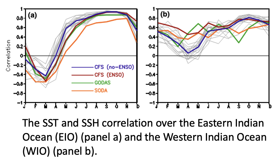
• Wang, H., Murtugudde, R. & Kumar, A. Evolution of Indian Ocean dipole and its forcing mechanisms in the absence of ENSO. Clim Dyn 47, 2481–2500 (2016). https://doi.org/10.1007/s00382-016-2977-y

Input datasets

1. ECCO Ocean Temperature and Salinity - Monthly Mean 0.5 Degree (Version 4 Release 4). DOI: https://doi.org/10.5067/ECG5M-OTS44
2. ECCO Sea Surface Height - Daily Mean 0.5 Degree (Version 4 Release 4b). DOI: https://doi.org/10.5067/ECG5D-SSH4B

Services and software used

1. NASA Harmony netcdf-to-Zarr
2. xarray, requests, json, pandas, numpy, matplotlib, s3fs
3. Various python utlities including the NASA harmony-py package

# Import various libraries

from matplotlib import pylab as plt
import xarray as xr
import numpy as np
import pandas as pd
import requests
import json
import time
import s3fs
import re

from datetime import datetime
from harmony import Client, Collection, Environment, Request

Identify the ShortName of the dataset of interest.

The shortname is an unique pointer for each NASA dataset.

ShortName = "ECCO_L4_SSH_05DEG_MONTHLY_V4R4B"

Set start and end dates

start_date = "1992-01-01"
end_date   = "2002-12-31"

# break it down into Year, Month, Day (and minutes and seconds if desired) 
# as inputs to harmony.py call using datetime()
start_year = 2002
start_month = 1
start_day = 1

end_year = 2017
end_month = 12
end_day = 31

Spatial bounds (Region of Interest) – Not used

westernmost_longitude = 100.
easternmost_longitude = 150.
northermost_latitude  = 30.
southernmost_latitude = 0.

Find the concept_id

response = requests.get(
    url='https://cmr.earthdata.nasa.gov/search/collections.umm_json', 
    params={'provider': "POCLOUD",
            'ShortName': ShortName,
            'page_size': 1}
)

ummc = response.json()['items'][0]

ccid = ummc['meta']['concept-id']

ccid

'C2129189405-POCLOUD'

NetCDF to Zarr transformation

Setup the harmony-py service call and execute a request

# using the the harmony.py service, set up the request and exectue it
ecco_collection = Collection(id=ccid)
time_range = {'start': datetime(start_year, start_month, start_day), 'stop': datetime(end_year, end_month, end_day)}
print(time_range)

harmony_client = Client(env=Environment.PROD)

# in this example set concatentae to 'False' because the monthly input time steps vary slightly
# (not always centered in the middle of month)
ecco_request = Request(collection=ecco_collection, temporal=time_range, format='application/x-zarr', concatenate='False')

# sumbit request and monitor job
ecco_job_id = harmony_client.submit(ecco_request)
print('\n Waiting for the job to finish. . .\n')
ecco_response = harmony_client.result_json(ecco_job_id, show_progress=True)
print("\n. . .DONE!")

{'start': datetime.datetime(2002, 1, 1, 0, 0), 'stop': datetime.datetime(2017, 12, 31, 0, 0)}

Waiting for the job to finish. . .

 [ Processing: 100% ] |###################################################| [|]

. . .DONE!

You can also wrap the creation of the Harmony request URL into one function. Shown here for legacy purposes (does not execute a Harmony request):

def get_harmony_url(ccid,start_date,end_date):
    """
    Parameters:
    ===========
    ccid: string
        concept_id of the datset
    date_range: list
        [start_data, end_date] 
        
    Return:
    =======
    url: the harmony URL used to perform the netcdf to zarr transformation
    """
    
    base = f"https://harmony.earthdata.nasa.gov/{ccid}"
    hreq = f"{base}/ogc-api-coverages/1.0.0/collections/all/coverage/rangeset"
    rurl = f"{hreq}?format=application/x-zarr"

    #print(rurl)

    subs = '&'.join([f'subset=time("{start_date}T00:00:00.000Z":"{end_date}T23:59:59.999Z")']) 
    #subs = subs + '&' + '&'.join([f'subset=lat({southernmost_latitude}:{northermost_latitude})'])
    #subs = subs + '&' + '&'.join([f'subset=lon({westernmost_longitude}:{easternmost_longitude})'])

    rurl = f"{rurl}&{subs}"
    return rurl

ccid='C2129189405-POCLOUD'
print(get_harmony_url(ccid,start_date,end_date))

# this is the way you would execute it
# response = requests.get(url=rurl).json()

https://harmony.earthdata.nasa.gov/C2129189405-POCLOUD/ogc-api-coverages/1.0.0/collections/all/coverage/rangeset?format=application/x-zarr&subset=time("1992-01-01T00:00:00.000Z":"2002-12-31T23:59:59.999Z")

Access the staged cloud datasets over native AWS interfaces

print(ecco_response['message'])
with requests.get(ecco_response['links'][2]['href']) as r:
    creds = r.json()

print( creds.keys() )
print("AWS credentials expire on: ", creds['Expiration'] )

The job has completed successfully. Contains results in AWS S3. Access from AWS us-west-2 with keys from https://harmony.earthdata.nasa.gov/cloud-access.sh
dict_keys(['AccessKeyId', 'SecretAccessKey', 'SessionToken', 'Expiration'])
AWS credentials expire on:  2022-05-03T08:45:27.000Z

List zarr datasets with s3fs

s3_dir = ecco_response['links'][3]['href']

print("root directory:", s3_dir)

s3_urls = [u['href'] for u in ecco_response['links'][4:-1]]

# sort the URLs in time order
s3_urls.sort()

print(s3_urls[0])

s3 = s3fs.S3FileSystem(
    key=creds['AccessKeyId'],
    secret=creds['SecretAccessKey'],
    token=creds['SessionToken'],
    client_kwargs={'region_name':'us-west-2'},
)

len(s3.ls(s3_dir))

root directory: s3://harmony-prod-staging/public/harmony/netcdf-to-zarr/0164d106-f8f0-431e-926c-c7d3f5f0575e/
s3://harmony-prod-staging/public/harmony/netcdf-to-zarr/0164d106-f8f0-431e-926c-c7d3f5f0575e/SEA_SURFACE_HEIGHT_mon_mean_2001-12_ECCO_V4r4b_latlon_0p50deg.zarr

193

Open datasets with xarray()

ds0 = xr.open_zarr(s3.get_mapper(s3_urls[0]), decode_cf=True, mask_and_scale=True)
ds0

<xarray.Dataset>
Dimensions:         (time: 1, latitude: 360, longitude: 720, nv: 2)
Coordinates:
  * latitude        (latitude) float32 -89.75 -89.25 -88.75 ... 89.25 89.75
    latitude_bnds   (latitude, nv) float32 dask.array<chunksize=(360, 2), meta=np.ndarray>
  * longitude       (longitude) float32 -179.8 -179.2 -178.8 ... 179.2 179.8
    longitude_bnds  (longitude, nv) float32 dask.array<chunksize=(720, 2), meta=np.ndarray>
  * time            (time) datetime64[ns] 2001-12-16T12:00:00
    time_bnds       (time, nv) datetime64[ns] dask.array<chunksize=(1, 2), meta=np.ndarray>
Dimensions without coordinates: nv
Data variables:
    SSH             (time, latitude, longitude) float32 dask.array<chunksize=(1, 360, 720), meta=np.ndarray>
    SSHIBC          (time, latitude, longitude) float32 dask.array<chunksize=(1, 360, 720), meta=np.ndarray>
    SSHNOIBC        (time, latitude, longitude) float32 dask.array<chunksize=(1, 360, 720), meta=np.ndarray>
Attributes: (12/57)
    Conventions:                  CF-1.8, ACDD-1.3
    acknowledgement:              This research was carried out by the Jet Pr...
    author:                       Ou Wang and Ian Fenty
    cdm_data_type:                Grid
    comment:                      Fields provided on a regular lat-lon grid. ...
    coordinates_comment:          Note: the global 'coordinates' attribute de...
    ...                           ...
    time_coverage_duration:       P1M
    time_coverage_end:            2002-01-01T00:00:00
    time_coverage_resolution:     P1M
    time_coverage_start:          2001-12-01T00:00:00
    title:                        ECCO Sea Surface Height - Monthly Mean 0.5 ...
    uuid:                         cd67c8ad-0f9e-4cf7-a3c3-4ac4d6016ea5

xarray.Dataset

• Dimensions:
  • time: 1
  • latitude: 360
  • longitude: 720
  • nv: 2
• Coordinates: (6)
  • latitude
    (latitude)
    float32
    -89.75 -89.25 ... 89.25 89.75

    axis :

    Y

    bounds :

    latitude_bnds

    comment :

    uniform grid spacing from -89.75 to 89.75 by 0.5

    coverage_content_type :

    coordinate

    long_name :

    latitude at grid cell center

    standard_name :

    latitude

    units :

    degrees_north

    array([-89.75, -89.25, -88.75, ...,  88.75,  89.25,  89.75], dtype=float32)

  • latitude_bnds
    (latitude, nv)
    float32
    dask.array<chunksize=(360, 2), meta=np.ndarray>

    coverage_content_type :

    coordinate

    long_name :

    latitude bounds grid cells

    Array Chunk Bytes 2.81 kiB 2.81 kiB Shape (360, 2) (360, 2) Count 2 Tasks 1 Chunks Type float32 numpy.ndarray

  • longitude
    (longitude)
    float32
    -179.8 -179.2 ... 179.2 179.8

    axis :

    X

    bounds :

    longitude_bnds

    comment :

    uniform grid spacing from -179.75 to 179.75 by 0.5

    coverage_content_type :

    coordinate

    long_name :

    longitude at grid cell center

    standard_name :

    longitude

    units :

    degrees_east

    array([-179.75, -179.25, -178.75, ...,  178.75,  179.25,  179.75],
          dtype=float32)

  • longitude_bnds
    (longitude, nv)
    float32
    dask.array<chunksize=(720, 2), meta=np.ndarray>

    coverage_content_type :

    coordinate

    long_name :

    longitude bounds grid cells

    Array Chunk Bytes 5.62 kiB 5.62 kiB Shape (720, 2) (720, 2) Count 2 Tasks 1 Chunks Type float32 numpy.ndarray

  • time
    (time)
    datetime64[ns]
    2001-12-16T12:00:00

    axis :

    T

    bounds :

    time_bnds

    coverage_content_type :

    coordinate

    long_name :

    center time of averaging period

    standard_name :

    time

    array(['2001-12-16T12:00:00.000000000'], dtype='datetime64[ns]')

  • time_bnds
    (time, nv)
    datetime64[ns]
    dask.array<chunksize=(1, 2), meta=np.ndarray>

    comment :

    Start and end times of averaging period.

    coverage_content_type :

    coordinate

    long_name :

    time bounds of averaging period

    Array Chunk Bytes 16 B 16 B Shape (1, 2) (1, 2) Count 2 Tasks 1 Chunks Type datetime64[ns] numpy.ndarray

• Data variables: (3)
  • SSH
    (time, latitude, longitude)
    float32
    dask.array<chunksize=(1, 360, 720), meta=np.ndarray>

    comment :

    Dynamic sea surface height anomaly above the geoid, suitable for comparisons with altimetry sea surface height data products that apply the inverse barometer (IB) correction. Note: SSH is calculated by correcting model sea level anomaly ETAN for three effects: a) global mean steric sea level changes related to density changes in the Boussinesq volume-conserving model (Greatbatch correction, see sterGloH), b) the inverted barometer (IB) effect (see SSHIBC) and c) sea level displacement due to sea-ice and snow pressure loading (see sIceLoad). SSH can be compared with the similarly-named SSH variable in previous ECCO products that did not include atmospheric pressure loading (e.g., Version 4 Release 3). Use SSHNOIBC for comparisons with altimetry data products that do NOT apply the IB correction.

    coverage_content_type :

    modelResult

    long_name :

    Dynamic sea surface height anomaly

    standard_name :

    sea_surface_height_above_geoid

    units :

    m

    valid_max :

    1.4207719564437866

    valid_min :

    -1.8805772066116333

    Array Chunk Bytes 0.99 MiB 0.99 MiB Shape (1, 360, 720) (1, 360, 720) Count 2 Tasks 1 Chunks Type float32 numpy.ndarray

  • SSHIBC
    (time, latitude, longitude)
    float32
    dask.array<chunksize=(1, 360, 720), meta=np.ndarray>

    comment :

    Not an SSH itself, but a correction to model sea level anomaly (ETAN) required to account for the static part of sea surface displacement by atmosphere pressure loading: SSH = SSHNOIBC - SSHIBC. Note: Use SSH for model-data comparisons with altimetry data products that DO apply the IB correction and SSHNOIBC for comparisons with altimetry data products that do NOT apply the IB correction.

    coverage_content_type :

    modelResult

    long_name :

    The inverted barometer (IB) correction to sea surface height due to atmospheric pressure loading

    units :

    m

    valid_max :

    0.5245633721351624

    valid_min :

    -0.3014216423034668

    Array Chunk Bytes 0.99 MiB 0.99 MiB Shape (1, 360, 720) (1, 360, 720) Count 2 Tasks 1 Chunks Type float32 numpy.ndarray

  • SSHNOIBC
    (time, latitude, longitude)
    float32
    dask.array<chunksize=(1, 360, 720), meta=np.ndarray>

    comment :

    Sea surface height anomaly above the geoid without the inverse barometer (IB) correction, suitable for comparisons with altimetry sea surface height data products that do NOT apply the inverse barometer (IB) correction. Note: SSHNOIBC is calculated by correcting model sea level anomaly ETAN for two effects: a) global mean steric sea level changes related to density changes in the Boussinesq volume-conserving model (Greatbatch correction, see sterGloH), b) sea level displacement due to sea-ice and snow pressure loading (see sIceLoad). In ECCO Version 4 Release 4b the model is forced with atmospheric pressure loading. SSHNOIBC does not correct for the static part of the effect of atmosphere pressure loading on sea surface height (the so-called inverse barometer (IB) correction). Use SSH for comparisons with altimetry data products that DO apply the IB correction.

    coverage_content_type :

    modelResult

    long_name :

    Sea surface height anomaly without the inverted barometer (IB) correction

    units :

    m

    valid_max :

    1.4550364017486572

    valid_min :

    -1.6654272079467773

    Array Chunk Bytes 0.99 MiB 0.99 MiB Shape (1, 360, 720) (1, 360, 720) Count 2 Tasks 1 Chunks Type float32 numpy.ndarray

• Attributes: (57)

  Conventions :

  CF-1.8, ACDD-1.3

  acknowledgement :

  This research was carried out by the Jet Propulsion Laboratory, managed by the California Institute of Technology under a contract with the National Aeronautics and Space Administration.

  author :

  Ou Wang and Ian Fenty

  cdm_data_type :

  Grid

  comment :

  Fields provided on a regular lat-lon grid. They have been mapped to the regular lat-lon grid from the original ECCO lat-lon-cap 90 (llc90) native model grid. SSH (dynamic sea surface height) = SSHNOIBC (dynamic sea surface without the inverse barometer correction) - SSHIBC (inverse barometer correction). The inverted barometer correction accounts for variations in sea surface height due to atmospheric pressure variations.

  coordinates_comment :

  Note: the global 'coordinates' attribute describes auxillary coordinates.

  creator_email :

  ecco-group@mit.edu

  creator_institution :

  NASA Jet Propulsion Laboratory (JPL)

  creator_name :

  ECCO Consortium

  creator_type :

  group

  creator_url :

  https://ecco-group.org

  date_created :

  2021-09-26T15:28:22

  date_issued :

  2021-09-26T15:28:22

  date_metadata_modified :

  2021-09-26T15:28:22

  date_modified :

  2021-09-26T15:28:22

  geospatial_bounds_crs :

  EPSG:4326

  geospatial_lat_max :

  90.0

  geospatial_lat_min :

  -90.0

  geospatial_lat_resolution :

  0.5

  geospatial_lat_units :

  degrees_north

  geospatial_lon_max :

  180.0

  geospatial_lon_min :

  -180.0

  geospatial_lon_resolution :

  0.5

  geospatial_lon_units :

  degrees_east

  history :

  Errata (Version 4, Release 4b) for Version 4, Release 4

  id :

  10.5067/ECG5M-SSH4B

  institution :

  NASA Jet Propulsion Laboratory (JPL)

  instrument_vocabulary :

  GCMD instrument keywords

  keywords :

  EARTH SCIENCE SERVICES > MODELS > EARTH SCIENCE REANALYSES/ASSIMILATION MODELS, EARTH SCIENCE > OCEANS > SEA SURFACE TOPOGRAPHY > SEA SURFACE HEIGHT

  keywords_vocabulary :

  NASA Global Change Master Directory (GCMD) Science Keywords

  license :

  Public Domain

  metadata_link :

  https://cmr.earthdata.nasa.gov/search/collections.umm_json?ShortName=ECCO_L4_SSH_05DEG_MONTHLY_V4R4B

  naming_authority :

  gov.nasa.jpl

  platform :

  ERS-1/2, TOPEX/Poseidon, Geosat Follow-On (GFO), ENVISAT, Jason-1, Jason-2, CryoSat-2, SARAL/AltiKa, Jason-3, AVHRR, Aquarius, SSM/I, SSMIS, GRACE, DTU17MDT, Argo, WOCE, GO-SHIP, MEOP, Ice Tethered Profilers (ITP)

  platform_vocabulary :

  GCMD platform keywords

  processing_level :

  L4

  product_name :

  SEA_SURFACE_HEIGHT_mon_mean_2001-12_ECCO_V4r4b_latlon_0p50deg.nc

  product_time_coverage_end :

  2018-01-01T00:00:00

  product_time_coverage_start :

  1992-01-01T12:00:00

  product_version :

  Version 4, Release 4b (Errata for Version 4, Release 4)

  program :

  NASA Physical Oceanography, Cryosphere, Modeling, Analysis, and Prediction (MAP)

  project :

  Estimating the Circulation and Climate of the Ocean (ECCO)

  publisher_email :

  podaac@podaac.jpl.nasa.gov

  publisher_institution :

  PO.DAAC

  publisher_name :

  Physical Oceanography Distributed Active Archive Center (PO.DAAC)

  publisher_type :

  institution

  publisher_url :

  https://podaac.jpl.nasa.gov

  references :

  ECCO Consortium, Fukumori, I., Wang, O., Fenty, I., Forget, G., Heimbach, P., & Ponte, R. M. 2020. Synopsis of the ECCO Central Production Global Ocean and Sea-Ice State Estimate (Version 4 Release 4). doi:10.5281/zenodo.3765928

  source :

  The ECCO V4r4b state estimate was produced by fitting a free-running solution of the MITgcm (checkpoint 66g) to satellite and in situ observational data in a least squares sense using the adjoint method

  standard_name_vocabulary :

  NetCDF Climate and Forecast (CF) Metadata Convention

  summary :

  This product (Version 4, Release 4b) is the errata for Version 4 Release 4. The errata document is available at https://ecco-group.org/docs/ECCO_V4r4_errata.pdf. This dataset provides monthly-averaged dynamic sea surface height interpolated to a regular 0.5-degree grid from the ECCO Version 4 Release 4 (V4r4b) ocean and sea-ice state estimate. Estimating the Circulation and Climate of the Ocean (ECCO) state estimates are dynamically and kinematically-consistent reconstructions of the three-dimensional, time-evolving ocean, sea-ice, and surface atmospheric states. ECCO V4r4b is a free-running solution of a global, nominally 1-degree configuration of the MIT general circulation model (MITgcm) that has been fit to observations in a least-squares sense. Observational data constraints used in V4r4b include sea surface height (SSH) from satellite altimeters [ERS-1/2, TOPEX/Poseidon, GFO, ENVISAT, Jason-1,2,3, CryoSat-2, and SARAL/AltiKa]; sea surface temperature (SST) from satellite radiometers [AVHRR], sea surface salinity (SSS) from the Aquarius satellite radiometer/scatterometer, ocean bottom pressure (OBP) from the GRACE satellite gravimeter; sea-ice concentration from satellite radiometers [SSM/I and SSMIS], and in-situ ocean temperature and salinity measured with conductivity-temperature-depth (CTD) sensors and expendable bathythermographs (XBTs) from several programs [e.g., WOCE, GO-SHIP, Argo, and others] and platforms [e.g., research vessels, gliders, moorings, ice-tethered profilers, and instrumented pinnipeds]. V4r4b covers the period 1992-01-01T12:00:00 to 2018-01-01T00:00:00.

  time_coverage_duration :

  P1M

  time_coverage_end :

  2002-01-01T00:00:00

  time_coverage_resolution :

  P1M

  time_coverage_start :

  2001-12-01T00:00:00

  title :

  ECCO Sea Surface Height - Monthly Mean 0.5 Degree (Version 4 Release 4b)

  uuid :

  cd67c8ad-0f9e-4cf7-a3c3-4ac4d6016ea5

Concatenate all granules (datasets) via a loop

ssh_ds = xr.concat([xr.open_zarr(s3.get_mapper(u)) for u in s3_urls], dim="time", coords='minimal')
ssh_ds
#ssh_ds_group = xr.concat([xr.open_zarr(s3.get_mapper(u)) for u in s3_urls], dim="time", coords='minimal').groupby('time.month')

<xarray.Dataset>
Dimensions:         (time: 193, latitude: 360, longitude: 720, nv: 2)
Coordinates:
  * latitude        (latitude) float32 -89.75 -89.25 -88.75 ... 89.25 89.75
    latitude_bnds   (latitude, nv) float32 -90.0 -89.5 -89.5 ... 89.5 89.5 90.0
  * longitude       (longitude) float32 -179.8 -179.2 -178.8 ... 179.2 179.8
    longitude_bnds  (longitude, nv) float32 -180.0 -179.5 -179.5 ... 179.5 180.0
  * time            (time) datetime64[ns] 2001-12-16T12:00:00 ... 2017-12-16T...
    time_bnds       (time, nv) datetime64[ns] dask.array<chunksize=(1, 2), meta=np.ndarray>
Dimensions without coordinates: nv
Data variables:
    SSH             (time, latitude, longitude) float32 dask.array<chunksize=(1, 360, 720), meta=np.ndarray>
    SSHIBC          (time, latitude, longitude) float32 dask.array<chunksize=(1, 360, 720), meta=np.ndarray>
    SSHNOIBC        (time, latitude, longitude) float32 dask.array<chunksize=(1, 360, 720), meta=np.ndarray>
Attributes: (12/57)
    Conventions:                  CF-1.8, ACDD-1.3
    acknowledgement:              This research was carried out by the Jet Pr...
    author:                       Ou Wang and Ian Fenty
    cdm_data_type:                Grid
    comment:                      Fields provided on a regular lat-lon grid. ...
    coordinates_comment:          Note: the global 'coordinates' attribute de...
    ...                           ...
    time_coverage_duration:       P1M
    time_coverage_end:            2002-01-01T00:00:00
    time_coverage_resolution:     P1M
    time_coverage_start:          2001-12-01T00:00:00
    title:                        ECCO Sea Surface Height - Monthly Mean 0.5 ...
    uuid:                         cd67c8ad-0f9e-4cf7-a3c3-4ac4d6016ea5

xarray.Dataset

• Dimensions:
  • time: 193
  • latitude: 360
  • longitude: 720
  • nv: 2
• Coordinates: (6)
  • latitude
    (latitude)
    float32
    -89.75 -89.25 ... 89.25 89.75

    axis :

    Y

    bounds :

    latitude_bnds

    comment :

    uniform grid spacing from -89.75 to 89.75 by 0.5

    coverage_content_type :

    coordinate

    long_name :

    latitude at grid cell center

    standard_name :

    latitude

    units :

    degrees_north

    array([-89.75, -89.25, -88.75, ...,  88.75,  89.25,  89.75], dtype=float32)

  • latitude_bnds
    (latitude, nv)
    float32
    -90.0 -89.5 -89.5 ... 89.5 90.0

    coverage_content_type :

    coordinate

    long_name :

    latitude bounds grid cells

    array([[-90. , -89.5],
           [-89.5, -89. ],
           [-89. , -88.5],
           [-88.5, -88. ],
           [-88. , -87.5],
           [-87.5, -87. ],
           [-87. , -86.5],
           [-86.5, -86. ],
           [-86. , -85.5],
           [-85.5, -85. ],
           [-85. , -84.5],
           [-84.5, -84. ],
           [-84. , -83.5],
           [-83.5, -83. ],
           [-83. , -82.5],
           [-82.5, -82. ],
           [-82. , -81.5],
           [-81.5, -81. ],
           [-81. , -80.5],
           [-80.5, -80. ],
    ...
           [ 80. ,  80.5],
           [ 80.5,  81. ],
           [ 81. ,  81.5],
           [ 81.5,  82. ],
           [ 82. ,  82.5],
           [ 82.5,  83. ],
           [ 83. ,  83.5],
           [ 83.5,  84. ],
           [ 84. ,  84.5],
           [ 84.5,  85. ],
           [ 85. ,  85.5],
           [ 85.5,  86. ],
           [ 86. ,  86.5],
           [ 86.5,  87. ],
           [ 87. ,  87.5],
           [ 87.5,  88. ],
           [ 88. ,  88.5],
           [ 88.5,  89. ],
           [ 89. ,  89.5],
           [ 89.5,  90. ]], dtype=float32)

  • longitude
    (longitude)
    float32
    -179.8 -179.2 ... 179.2 179.8

    axis :

    X

    bounds :

    longitude_bnds

    comment :

    uniform grid spacing from -179.75 to 179.75 by 0.5

    coverage_content_type :

    coordinate

    long_name :

    longitude at grid cell center

    standard_name :

    longitude

    units :

    degrees_east

    array([-179.75, -179.25, -178.75, ...,  178.75,  179.25,  179.75],
          dtype=float32)

  • longitude_bnds
    (longitude, nv)
    float32
    -180.0 -179.5 ... 179.5 180.0

    coverage_content_type :

    coordinate

    long_name :

    longitude bounds grid cells

    array([[-180. , -179.5],
           [-179.5, -179. ],
           [-179. , -178.5],
           ...,
           [ 178.5,  179. ],
           [ 179. ,  179.5],
           [ 179.5,  180. ]], dtype=float32)

  • time
    (time)
    datetime64[ns]
    2001-12-16T12:00:00 ... 2017-12-...

    axis :

    T

    bounds :

    time_bnds

    coverage_content_type :

    coordinate

    long_name :

    center time of averaging period

    standard_name :

    time

    array(['2001-12-16T12:00:00.000000000', '2002-01-16T12:00:00.000000000',
           '2002-02-15T00:00:00.000000000', '2002-03-16T12:00:00.000000000',
           '2002-04-16T00:00:00.000000000', '2002-05-16T12:00:00.000000000',
           '2002-06-16T00:00:00.000000000', '2002-07-16T12:00:00.000000000',
           '2002-08-16T12:00:00.000000000', '2002-09-16T00:00:00.000000000',
           '2002-10-16T12:00:00.000000000', '2002-11-16T00:00:00.000000000',
           '2002-12-16T12:00:00.000000000', '2003-01-16T12:00:00.000000000',
           '2003-02-15T00:00:00.000000000', '2003-03-16T12:00:00.000000000',
           '2003-04-16T00:00:00.000000000', '2003-05-16T12:00:00.000000000',
           '2003-06-16T00:00:00.000000000', '2003-07-16T12:00:00.000000000',
           '2003-08-16T12:00:00.000000000', '2003-09-16T00:00:00.000000000',
           '2003-10-16T12:00:00.000000000', '2003-11-16T00:00:00.000000000',
           '2003-12-16T12:00:00.000000000', '2004-01-16T12:00:00.000000000',
           '2004-02-15T12:00:00.000000000', '2004-03-16T12:00:00.000000000',
           '2004-04-16T00:00:00.000000000', '2004-05-16T12:00:00.000000000',
           '2004-06-16T00:00:00.000000000', '2004-07-16T12:00:00.000000000',
           '2004-08-16T12:00:00.000000000', '2004-09-16T00:00:00.000000000',
           '2004-10-16T12:00:00.000000000', '2004-11-16T00:00:00.000000000',
           '2004-12-16T12:00:00.000000000', '2005-01-16T12:00:00.000000000',
           '2005-02-15T00:00:00.000000000', '2005-03-16T12:00:00.000000000',
           '2005-04-16T00:00:00.000000000', '2005-05-16T12:00:00.000000000',
           '2005-06-16T00:00:00.000000000', '2005-07-16T12:00:00.000000000',
           '2005-08-16T12:00:00.000000000', '2005-09-16T00:00:00.000000000',
           '2005-10-16T12:00:00.000000000', '2005-11-16T00:00:00.000000000',
           '2005-12-16T12:00:00.000000000', '2006-01-16T12:00:00.000000000',
           '2006-02-15T00:00:00.000000000', '2006-03-16T12:00:00.000000000',
           '2006-04-16T00:00:00.000000000', '2006-05-16T12:00:00.000000000',
           '2006-06-16T00:00:00.000000000', '2006-07-16T12:00:00.000000000',
           '2006-08-16T12:00:00.000000000', '2006-09-16T00:00:00.000000000',
           '2006-10-16T12:00:00.000000000', '2006-11-16T00:00:00.000000000',
           '2006-12-16T12:00:00.000000000', '2007-01-16T12:00:00.000000000',
           '2007-02-15T00:00:00.000000000', '2007-03-16T12:00:00.000000000',
           '2007-04-16T00:00:00.000000000', '2007-05-16T12:00:00.000000000',
           '2007-06-16T00:00:00.000000000', '2007-07-16T12:00:00.000000000',
           '2007-08-16T12:00:00.000000000', '2007-09-16T00:00:00.000000000',
           '2007-10-16T12:00:00.000000000', '2007-11-16T00:00:00.000000000',
           '2007-12-16T12:00:00.000000000', '2008-01-16T12:00:00.000000000',
           '2008-02-15T12:00:00.000000000', '2008-03-16T12:00:00.000000000',
           '2008-04-16T00:00:00.000000000', '2008-05-16T12:00:00.000000000',
           '2008-06-16T00:00:00.000000000', '2008-07-16T12:00:00.000000000',
           '2008-08-16T12:00:00.000000000', '2008-09-16T00:00:00.000000000',
           '2008-10-16T12:00:00.000000000', '2008-11-16T00:00:00.000000000',
           '2008-12-16T12:00:00.000000000', '2009-01-16T12:00:00.000000000',
           '2009-02-15T00:00:00.000000000', '2009-03-16T12:00:00.000000000',
           '2009-04-16T00:00:00.000000000', '2009-05-16T12:00:00.000000000',
           '2009-06-16T00:00:00.000000000', '2009-07-16T12:00:00.000000000',
           '2009-08-16T12:00:00.000000000', '2009-09-16T00:00:00.000000000',
           '2009-10-16T12:00:00.000000000', '2009-11-16T00:00:00.000000000',
           '2009-12-16T12:00:00.000000000', '2010-01-16T12:00:00.000000000',
           '2010-02-15T00:00:00.000000000', '2010-03-16T12:00:00.000000000',
           '2010-04-16T00:00:00.000000000', '2010-05-16T12:00:00.000000000',
           '2010-06-16T00:00:00.000000000', '2010-07-16T12:00:00.000000000',
           '2010-08-16T12:00:00.000000000', '2010-09-16T00:00:00.000000000',
           '2010-10-16T12:00:00.000000000', '2010-11-16T00:00:00.000000000',
           '2010-12-16T12:00:00.000000000', '2011-01-16T12:00:00.000000000',
           '2011-02-15T00:00:00.000000000', '2011-03-16T12:00:00.000000000',
           '2011-04-16T00:00:00.000000000', '2011-05-16T12:00:00.000000000',
           '2011-06-16T00:00:00.000000000', '2011-07-16T12:00:00.000000000',
           '2011-08-16T12:00:00.000000000', '2011-09-16T00:00:00.000000000',
           '2011-10-16T12:00:00.000000000', '2011-11-16T00:00:00.000000000',
           '2011-12-16T12:00:00.000000000', '2012-01-16T12:00:00.000000000',
           '2012-02-15T12:00:00.000000000', '2012-03-16T12:00:00.000000000',
           '2012-04-16T00:00:00.000000000', '2012-05-16T12:00:00.000000000',
           '2012-06-16T00:00:00.000000000', '2012-07-16T12:00:00.000000000',
           '2012-08-16T12:00:00.000000000', '2012-09-16T00:00:00.000000000',
           '2012-10-16T12:00:00.000000000', '2012-11-16T00:00:00.000000000',
           '2012-12-16T12:00:00.000000000', '2013-01-16T12:00:00.000000000',
           '2013-02-15T00:00:00.000000000', '2013-03-16T12:00:00.000000000',
           '2013-04-16T00:00:00.000000000', '2013-05-16T12:00:00.000000000',
           '2013-06-16T00:00:00.000000000', '2013-07-16T12:00:00.000000000',
           '2013-08-16T12:00:00.000000000', '2013-09-16T00:00:00.000000000',
           '2013-10-16T12:00:00.000000000', '2013-11-16T00:00:00.000000000',
           '2013-12-16T12:00:00.000000000', '2014-01-16T12:00:00.000000000',
           '2014-02-15T00:00:00.000000000', '2014-03-16T12:00:00.000000000',
           '2014-04-16T00:00:00.000000000', '2014-05-16T12:00:00.000000000',
           '2014-06-16T00:00:00.000000000', '2014-07-16T12:00:00.000000000',
           '2014-08-16T12:00:00.000000000', '2014-09-16T00:00:00.000000000',
           '2014-10-16T12:00:00.000000000', '2014-11-16T00:00:00.000000000',
           '2014-12-16T12:00:00.000000000', '2015-01-16T12:00:00.000000000',
           '2015-02-15T00:00:00.000000000', '2015-03-16T12:00:00.000000000',
           '2015-04-16T00:00:00.000000000', '2015-05-16T12:00:00.000000000',
           '2015-06-16T00:00:00.000000000', '2015-07-16T12:00:00.000000000',
           '2015-08-16T12:00:00.000000000', '2015-09-16T00:00:00.000000000',
           '2015-10-16T12:00:00.000000000', '2015-11-16T00:00:00.000000000',
           '2015-12-16T12:00:00.000000000', '2016-01-16T12:00:00.000000000',
           '2016-02-15T12:00:00.000000000', '2016-03-16T12:00:00.000000000',
           '2016-04-16T00:00:00.000000000', '2016-05-16T12:00:00.000000000',
           '2016-06-16T00:00:00.000000000', '2016-07-16T12:00:00.000000000',
           '2016-08-16T12:00:00.000000000', '2016-09-16T00:00:00.000000000',
           '2016-10-16T12:00:00.000000000', '2016-11-16T00:00:00.000000000',
           '2016-12-16T12:00:00.000000000', '2017-01-16T12:00:00.000000000',
           '2017-02-15T00:00:00.000000000', '2017-03-16T12:00:00.000000000',
           '2017-04-16T00:00:00.000000000', '2017-05-16T12:00:00.000000000',
           '2017-06-16T00:00:00.000000000', '2017-07-16T12:00:00.000000000',
           '2017-08-16T12:00:00.000000000', '2017-09-16T00:00:00.000000000',
           '2017-10-16T12:00:00.000000000', '2017-11-16T00:00:00.000000000',
           '2017-12-16T06:00:00.000000000'], dtype='datetime64[ns]')

  • time_bnds
    (time, nv)
    datetime64[ns]
    dask.array<chunksize=(1, 2), meta=np.ndarray>

    comment :

    Start and end times of averaging period.

    coverage_content_type :

    coordinate

    long_name :

    time bounds of averaging period

    Array Chunk Bytes 3.02 kiB 16 B Shape (193, 2) (1, 2) Count 579 Tasks 193 Chunks Type datetime64[ns] numpy.ndarray

• Data variables: (3)
  • SSH
    (time, latitude, longitude)
    float32
    dask.array<chunksize=(1, 360, 720), meta=np.ndarray>

    comment :

    Dynamic sea surface height anomaly above the geoid, suitable for comparisons with altimetry sea surface height data products that apply the inverse barometer (IB) correction. Note: SSH is calculated by correcting model sea level anomaly ETAN for three effects: a) global mean steric sea level changes related to density changes in the Boussinesq volume-conserving model (Greatbatch correction, see sterGloH), b) the inverted barometer (IB) effect (see SSHIBC) and c) sea level displacement due to sea-ice and snow pressure loading (see sIceLoad). SSH can be compared with the similarly-named SSH variable in previous ECCO products that did not include atmospheric pressure loading (e.g., Version 4 Release 3). Use SSHNOIBC for comparisons with altimetry data products that do NOT apply the IB correction.

    coverage_content_type :

    modelResult

    long_name :

    Dynamic sea surface height anomaly

    standard_name :

    sea_surface_height_above_geoid

    units :

    m

    valid_max :

    1.4207719564437866

    valid_min :

    -1.8805772066116333

    Array Chunk Bytes 190.83 MiB 0.99 MiB Shape (193, 360, 720) (1, 360, 720) Count 579 Tasks 193 Chunks Type float32 numpy.ndarray

  • SSHIBC
    (time, latitude, longitude)
    float32
    dask.array<chunksize=(1, 360, 720), meta=np.ndarray>

    comment :

    Not an SSH itself, but a correction to model sea level anomaly (ETAN) required to account for the static part of sea surface displacement by atmosphere pressure loading: SSH = SSHNOIBC - SSHIBC. Note: Use SSH for model-data comparisons with altimetry data products that DO apply the IB correction and SSHNOIBC for comparisons with altimetry data products that do NOT apply the IB correction.

    coverage_content_type :

    modelResult

    long_name :

    The inverted barometer (IB) correction to sea surface height due to atmospheric pressure loading

    units :

    m

    valid_max :

    0.5245633721351624

    valid_min :

    -0.3014216423034668

    Array Chunk Bytes 190.83 MiB 0.99 MiB Shape (193, 360, 720) (1, 360, 720) Count 579 Tasks 193 Chunks Type float32 numpy.ndarray

  • SSHNOIBC
    (time, latitude, longitude)
    float32
    dask.array<chunksize=(1, 360, 720), meta=np.ndarray>

    comment :

    Sea surface height anomaly above the geoid without the inverse barometer (IB) correction, suitable for comparisons with altimetry sea surface height data products that do NOT apply the inverse barometer (IB) correction. Note: SSHNOIBC is calculated by correcting model sea level anomaly ETAN for two effects: a) global mean steric sea level changes related to density changes in the Boussinesq volume-conserving model (Greatbatch correction, see sterGloH), b) sea level displacement due to sea-ice and snow pressure loading (see sIceLoad). In ECCO Version 4 Release 4b the model is forced with atmospheric pressure loading. SSHNOIBC does not correct for the static part of the effect of atmosphere pressure loading on sea surface height (the so-called inverse barometer (IB) correction). Use SSH for comparisons with altimetry data products that DO apply the IB correction.

    coverage_content_type :

    modelResult

    long_name :

    Sea surface height anomaly without the inverted barometer (IB) correction

    units :

    m

    valid_max :

    1.4550364017486572

    valid_min :

    -1.6654272079467773

    Array Chunk Bytes 190.83 MiB 0.99 MiB Shape (193, 360, 720) (1, 360, 720) Count 579 Tasks 193 Chunks Type float32 numpy.ndarray

• Attributes: (57)

  Conventions :

  CF-1.8, ACDD-1.3

  acknowledgement :

  This research was carried out by the Jet Propulsion Laboratory, managed by the California Institute of Technology under a contract with the National Aeronautics and Space Administration.

  author :

  Ou Wang and Ian Fenty

  cdm_data_type :

  Grid

  comment :

  Fields provided on a regular lat-lon grid. They have been mapped to the regular lat-lon grid from the original ECCO lat-lon-cap 90 (llc90) native model grid. SSH (dynamic sea surface height) = SSHNOIBC (dynamic sea surface without the inverse barometer correction) - SSHIBC (inverse barometer correction). The inverted barometer correction accounts for variations in sea surface height due to atmospheric pressure variations.

  coordinates_comment :

  Note: the global 'coordinates' attribute describes auxillary coordinates.

  creator_email :

  ecco-group@mit.edu

  creator_institution :

  NASA Jet Propulsion Laboratory (JPL)

  creator_name :

  ECCO Consortium

  creator_type :

  group

  creator_url :

  https://ecco-group.org

  date_created :

  2021-09-26T15:28:22

  date_issued :

  2021-09-26T15:28:22

  date_metadata_modified :

  2021-09-26T15:28:22

  date_modified :

  2021-09-26T15:28:22

  geospatial_bounds_crs :

  EPSG:4326

  geospatial_lat_max :

  90.0

  geospatial_lat_min :

  -90.0

  geospatial_lat_resolution :

  0.5

  geospatial_lat_units :

  degrees_north

  geospatial_lon_max :

  180.0

  geospatial_lon_min :

  -180.0

  geospatial_lon_resolution :

  0.5

  geospatial_lon_units :

  degrees_east

  history :

  Errata (Version 4, Release 4b) for Version 4, Release 4

  id :

  10.5067/ECG5M-SSH4B

  institution :

  NASA Jet Propulsion Laboratory (JPL)

  instrument_vocabulary :

  GCMD instrument keywords

  keywords :

  EARTH SCIENCE SERVICES > MODELS > EARTH SCIENCE REANALYSES/ASSIMILATION MODELS, EARTH SCIENCE > OCEANS > SEA SURFACE TOPOGRAPHY > SEA SURFACE HEIGHT

  keywords_vocabulary :

  NASA Global Change Master Directory (GCMD) Science Keywords

  license :

  Public Domain

  metadata_link :

  https://cmr.earthdata.nasa.gov/search/collections.umm_json?ShortName=ECCO_L4_SSH_05DEG_MONTHLY_V4R4B

  naming_authority :

  gov.nasa.jpl

  platform :

  ERS-1/2, TOPEX/Poseidon, Geosat Follow-On (GFO), ENVISAT, Jason-1, Jason-2, CryoSat-2, SARAL/AltiKa, Jason-3, AVHRR, Aquarius, SSM/I, SSMIS, GRACE, DTU17MDT, Argo, WOCE, GO-SHIP, MEOP, Ice Tethered Profilers (ITP)

  platform_vocabulary :

  GCMD platform keywords

  processing_level :

  L4

  product_name :

  SEA_SURFACE_HEIGHT_mon_mean_2001-12_ECCO_V4r4b_latlon_0p50deg.nc

  product_time_coverage_end :

  2018-01-01T00:00:00

  product_time_coverage_start :

  1992-01-01T12:00:00

  product_version :

  Version 4, Release 4b (Errata for Version 4, Release 4)

  program :

  NASA Physical Oceanography, Cryosphere, Modeling, Analysis, and Prediction (MAP)

  project :

  Estimating the Circulation and Climate of the Ocean (ECCO)

  publisher_email :

  podaac@podaac.jpl.nasa.gov

  publisher_institution :

  PO.DAAC

  publisher_name :

  Physical Oceanography Distributed Active Archive Center (PO.DAAC)

  publisher_type :

  institution

  publisher_url :

  https://podaac.jpl.nasa.gov

  references :

  ECCO Consortium, Fukumori, I., Wang, O., Fenty, I., Forget, G., Heimbach, P., & Ponte, R. M. 2020. Synopsis of the ECCO Central Production Global Ocean and Sea-Ice State Estimate (Version 4 Release 4). doi:10.5281/zenodo.3765928

  source :

  The ECCO V4r4b state estimate was produced by fitting a free-running solution of the MITgcm (checkpoint 66g) to satellite and in situ observational data in a least squares sense using the adjoint method

  standard_name_vocabulary :

  NetCDF Climate and Forecast (CF) Metadata Convention

  summary :

  This product (Version 4, Release 4b) is the errata for Version 4 Release 4. The errata document is available at https://ecco-group.org/docs/ECCO_V4r4_errata.pdf. This dataset provides monthly-averaged dynamic sea surface height interpolated to a regular 0.5-degree grid from the ECCO Version 4 Release 4 (V4r4b) ocean and sea-ice state estimate. Estimating the Circulation and Climate of the Ocean (ECCO) state estimates are dynamically and kinematically-consistent reconstructions of the three-dimensional, time-evolving ocean, sea-ice, and surface atmospheric states. ECCO V4r4b is a free-running solution of a global, nominally 1-degree configuration of the MIT general circulation model (MITgcm) that has been fit to observations in a least-squares sense. Observational data constraints used in V4r4b include sea surface height (SSH) from satellite altimeters [ERS-1/2, TOPEX/Poseidon, GFO, ENVISAT, Jason-1,2,3, CryoSat-2, and SARAL/AltiKa]; sea surface temperature (SST) from satellite radiometers [AVHRR], sea surface salinity (SSS) from the Aquarius satellite radiometer/scatterometer, ocean bottom pressure (OBP) from the GRACE satellite gravimeter; sea-ice concentration from satellite radiometers [SSM/I and SSMIS], and in-situ ocean temperature and salinity measured with conductivity-temperature-depth (CTD) sensors and expendable bathythermographs (XBTs) from several programs [e.g., WOCE, GO-SHIP, Argo, and others] and platforms [e.g., research vessels, gliders, moorings, ice-tethered profilers, and instrumented pinnipeds]. V4r4b covers the period 1992-01-01T12:00:00 to 2018-01-01T00:00:00.

  time_coverage_duration :

  P1M

  time_coverage_end :

  2002-01-01T00:00:00

  time_coverage_resolution :

  P1M

  time_coverage_start :

  2001-12-01T00:00:00

  title :

  ECCO Sea Surface Height - Monthly Mean 0.5 Degree (Version 4 Release 4b)

  uuid :

  cd67c8ad-0f9e-4cf7-a3c3-4ac4d6016ea5

Rinse and Repeat all steps for the second (ocean/salinity temperature) dataset

Run 2nd Harmony netCDF-to-Zarr call

ShortName = "ECCO_L4_TEMP_SALINITY_05DEG_MONTHLY_V4R4"

# 1) Find new concept_id for this dataset
response = requests.get(
        url='https://cmr.earthdata.nasa.gov/search/collections.umm_json', 
        params={'provider': "POCLOUD",
                'ShortName': ShortName,
                'page_size': 1}
)

ummc = response.json()['items'][0]
ccid = ummc['meta']['concept-id']

# using the the harmony.py service, set up the request and exectue it
ecco_collection = Collection(id=ccid)
time_range = {'start': datetime(start_year, start_month, start_day), 'stop': datetime(end_year, end_month, end_day)}

harmony_client = Client(env=Environment.PROD)

# in this example set concatentae to 'False' because the monthly input time steps vary slightly
# (not always centered in the middle of month)
ecco_request = Request(collection=ecco_collection, temporal=time_range, format='application/x-zarr', concatenate='False')

# sumbit request and monitor job
ecco_job_id = harmony_client.submit(ecco_request)
print('\nWaiting for the job to finish. . .\n')
ecco_response = harmony_client.result_json(ecco_job_id, show_progress=True)
print("\n. . .DONE!")

Waiting for the job to finish. . .

 [ Processing: 100% ] |###################################################| [|]

. . .DONE!

Read the S3 Zarr endpoints and aggregate to single Zarr

# 1) read the AWS credentials
print(ecco_response['message'])
with requests.get(ecco_response['links'][2]['href']) as r:
    creds = r.json()

print( creds.keys() )
print("AWS credentials expire on: ", creds['Expiration'] )


# 2) print root directory and read the s3 URLs into a list
s3_dir2 = ecco_response['links'][3]['href']
print("root directory:", s3_dir2)
s3_urls2 = [u['href'] for u in ecco_response['links'][4:-1]]

# sort the URLs in time order
s3_urls2.sort()

# 3) Autenticate AWS S3 credentials
s3 = s3fs.S3FileSystem(
    key=creds['AccessKeyId'],
    secret=creds['SecretAccessKey'],
    token=creds['SessionToken'],
    client_kwargs={'region_name':'us-west-2'},
)

# 4) Read and concatenate into a single Zarr dataset
temp_ds = xr.concat([xr.open_zarr(s3.get_mapper(u)) for u in s3_urls2], dim="time", coords='minimal')
#temp_ds_group = xr.concat([xr.open_zarr(s3.get_mapper(u)) for u in s3_urls2], dim="time", coords='minimal').groupby('time.month')

temp_ds

The job has completed successfully. Contains results in AWS S3. Access from AWS us-west-2 with keys from https://harmony.earthdata.nasa.gov/cloud-access.sh
dict_keys(['AccessKeyId', 'SecretAccessKey', 'SessionToken', 'Expiration'])
AWS credentials expire on:  2022-05-03T08:48:44.000Z
root directory: s3://harmony-prod-staging/public/harmony/netcdf-to-zarr/9dd5c9b3-84c4-48e5-907d-2bd21d92a60c/

<xarray.Dataset>
Dimensions:         (time: 193, Z: 50, latitude: 360, longitude: 720, nv: 2)
Coordinates:
  * Z               (Z) float32 -5.0 -15.0 -25.0 ... -5.461e+03 -5.906e+03
    Z_bnds          (Z, nv) float32 nan -10.0 -10.0 ... -5.678e+03 -6.134e+03
  * latitude        (latitude) float32 -89.75 -89.25 -88.75 ... 89.25 89.75
    latitude_bnds   (latitude, nv) float32 -90.0 -89.5 -89.5 ... 89.5 89.5 90.0
  * longitude       (longitude) float32 -179.8 -179.2 -178.8 ... 179.2 179.8
    longitude_bnds  (longitude, nv) float32 -180.0 -179.5 -179.5 ... 179.5 180.0
  * time            (time) datetime64[ns] 2001-12-16T12:00:00 ... 2017-12-16T...
    time_bnds       (time, nv) datetime64[ns] dask.array<chunksize=(1, 2), meta=np.ndarray>
Dimensions without coordinates: nv
Data variables:
    SALT            (time, Z, latitude, longitude) float32 dask.array<chunksize=(1, 50, 280, 280), meta=np.ndarray>
    THETA           (time, Z, latitude, longitude) float32 dask.array<chunksize=(1, 50, 280, 280), meta=np.ndarray>
Attributes: (12/62)
    Conventions:                     CF-1.8, ACDD-1.3
    acknowledgement:                 This research was carried out by the Jet...
    author:                          Ian Fenty and Ou Wang
    cdm_data_type:                   Grid
    comment:                         Fields provided on a regular lat-lon gri...
    coordinates_comment:             Note: the global 'coordinates' attribute...
    ...                              ...
    time_coverage_duration:          P1M
    time_coverage_end:               2002-01-01T00:00:00
    time_coverage_resolution:        P1M
    time_coverage_start:             2001-12-01T00:00:00
    title:                           ECCO Ocean Temperature and Salinity - Mo...
    uuid:                            7f718714-4159-11eb-8bbd-0cc47a3f819b

xarray.Dataset

• Dimensions:
  • time: 193
  • Z: 50
  • latitude: 360
  • longitude: 720
  • nv: 2
• Coordinates: (8)
  • Z
    (Z)
    float32
    -5.0 -15.0 ... -5.906e+03

    axis :

    Z

    bounds :

    Z_bnds

    comment :

    Non-uniform vertical spacing.

    coverage_content_type :

    coordinate

    long_name :

    depth of grid cell center

    positive :

    up

    standard_name :

    depth

    units :

    m

    array([-5.000000e+00, -1.500000e+01, -2.500000e+01, -3.500000e+01,
           -4.500000e+01, -5.500000e+01, -6.500000e+01, -7.500500e+01,
           -8.502500e+01, -9.509500e+01, -1.053100e+02, -1.158700e+02,
           -1.271500e+02, -1.397400e+02, -1.544700e+02, -1.724000e+02,
           -1.947350e+02, -2.227100e+02, -2.574700e+02, -2.999300e+02,
           -3.506800e+02, -4.099300e+02, -4.774700e+02, -5.527100e+02,
           -6.347350e+02, -7.224000e+02, -8.144700e+02, -9.097400e+02,
           -1.007155e+03, -1.105905e+03, -1.205535e+03, -1.306205e+03,
           -1.409150e+03, -1.517095e+03, -1.634175e+03, -1.765135e+03,
           -1.914150e+03, -2.084035e+03, -2.276225e+03, -2.491250e+03,
           -2.729250e+03, -2.990250e+03, -3.274250e+03, -3.581250e+03,
           -3.911250e+03, -4.264250e+03, -4.640250e+03, -5.039250e+03,
           -5.461250e+03, -5.906250e+03], dtype=float32)

  • Z_bnds
    (Z, nv)
    float32
    nan -10.0 ... -5.678e+03 -6.134e+03

    comment :

    One pair of bounds for each vertical level.

    coverage_content_type :

    coordinate

    long_name :

    depths of grid cell upper and lower interfaces

    array([[         nan,   -10.      ],
           [  -10.      ,   -20.      ],
           [  -20.      ,   -30.      ],
           [  -30.      ,   -40.      ],
           [  -40.      ,   -50.      ],
           [  -50.      ,   -60.      ],
           [  -60.      ,   -70.      ],
           [  -70.      ,   -80.01    ],
           [  -80.01    ,   -90.04    ],
           [  -90.04    ,  -100.15    ],
           [ -100.15    ,  -110.47    ],
           [ -110.47    ,  -121.270004],
           [ -121.270004,  -133.03    ],
           [ -133.03    ,  -146.45    ],
           [ -146.45    ,  -162.48999 ],
           [ -162.48999 ,  -182.31    ],
           [ -182.31    ,  -207.16    ],
           [ -207.16    ,  -238.26001 ],
           [ -238.26001 ,  -276.68    ],
           [ -276.68    ,  -323.18    ],
    ...
           [-1155.53    , -1255.54    ],
           [-1255.54    , -1356.87    ],
           [-1356.87    , -1461.4299  ],
           [-1461.4299  , -1572.7599  ],
           [-1572.7599  , -1695.5898  ],
           [-1695.5898  , -1834.6798  ],
           [-1834.6798  , -1993.6199  ],
           [-1993.6199  , -2174.45    ],
           [-2174.45    , -2378.      ],
           [-2378.      , -2604.5     ],
           [-2604.5     , -2854.      ],
           [-2854.      , -3126.5     ],
           [-3126.5     , -3422.      ],
           [-3422.      , -3740.5     ],
           [-3740.5     , -4082.      ],
           [-4082.      , -4446.5     ],
           [-4446.5     , -4834.      ],
           [-4834.      , -5244.5     ],
           [-5244.5     , -5678.      ],
           [-5678.      , -6134.5     ]], dtype=float32)

  • latitude
    (latitude)
    float32
    -89.75 -89.25 ... 89.25 89.75

    axis :

    Y

    bounds :

    latitude_bnds

    comment :

    uniform grid spacing from -89.75 to 89.75 by 0.5

    coverage_content_type :

    coordinate

    long_name :

    latitude at grid cell center

    standard_name :

    latitude

    units :

    degrees_north

    array([-89.75, -89.25, -88.75, ...,  88.75,  89.25,  89.75], dtype=float32)

  • latitude_bnds
    (latitude, nv)
    float32
    -90.0 -89.5 -89.5 ... 89.5 90.0

    coverage_content_type :

    coordinate

    long_name :

    latitude bounds grid cells

    array([[-90. , -89.5],
           [-89.5, -89. ],
           [-89. , -88.5],
           [-88.5, -88. ],
           [-88. , -87.5],
           [-87.5, -87. ],
           [-87. , -86.5],
           [-86.5, -86. ],
           [-86. , -85.5],
           [-85.5, -85. ],
           [-85. , -84.5],
           [-84.5, -84. ],
           [-84. , -83.5],
           [-83.5, -83. ],
           [-83. , -82.5],
           [-82.5, -82. ],
           [-82. , -81.5],
           [-81.5, -81. ],
           [-81. , -80.5],
           [-80.5, -80. ],
    ...
           [ 80. ,  80.5],
           [ 80.5,  81. ],
           [ 81. ,  81.5],
           [ 81.5,  82. ],
           [ 82. ,  82.5],
           [ 82.5,  83. ],
           [ 83. ,  83.5],
           [ 83.5,  84. ],
           [ 84. ,  84.5],
           [ 84.5,  85. ],
           [ 85. ,  85.5],
           [ 85.5,  86. ],
           [ 86. ,  86.5],
           [ 86.5,  87. ],
           [ 87. ,  87.5],
           [ 87.5,  88. ],
           [ 88. ,  88.5],
           [ 88.5,  89. ],
           [ 89. ,  89.5],
           [ 89.5,  90. ]], dtype=float32)

  • longitude
    (longitude)
    float32
    -179.8 -179.2 ... 179.2 179.8

    axis :

    X

    bounds :

    longitude_bnds

    comment :

    uniform grid spacing from -179.75 to 179.75 by 0.5

    coverage_content_type :

    coordinate

    long_name :

    longitude at grid cell center

    standard_name :

    longitude

    units :

    degrees_east

    array([-179.75, -179.25, -178.75, ...,  178.75,  179.25,  179.75],
          dtype=float32)

  • longitude_bnds
    (longitude, nv)
    float32
    -180.0 -179.5 ... 179.5 180.0

    coverage_content_type :

    coordinate

    long_name :

    longitude bounds grid cells

    array([[-180. , -179.5],
           [-179.5, -179. ],
           [-179. , -178.5],
           ...,
           [ 178.5,  179. ],
           [ 179. ,  179.5],
           [ 179.5,  180. ]], dtype=float32)

  • time
    (time)
    datetime64[ns]
    2001-12-16T12:00:00 ... 2017-12-...

    axis :

    T

    bounds :

    time_bnds

    coverage_content_type :

    coordinate

    long_name :

    center time of averaging period

    standard_name :

    time

    array(['2001-12-16T12:00:00.000000000', '2002-01-16T12:00:00.000000000',
           '2002-02-15T00:00:00.000000000', '2002-03-16T12:00:00.000000000',
           '2002-04-16T00:00:00.000000000', '2002-05-16T12:00:00.000000000',
           '2002-06-16T00:00:00.000000000', '2002-07-16T12:00:00.000000000',
           '2002-08-16T12:00:00.000000000', '2002-09-16T00:00:00.000000000',
           '2002-10-16T12:00:00.000000000', '2002-11-16T00:00:00.000000000',
           '2002-12-16T12:00:00.000000000', '2003-01-16T12:00:00.000000000',
           '2003-02-15T00:00:00.000000000', '2003-03-16T12:00:00.000000000',
           '2003-04-16T00:00:00.000000000', '2003-05-16T12:00:00.000000000',
           '2003-06-16T00:00:00.000000000', '2003-07-16T12:00:00.000000000',
           '2003-08-16T12:00:00.000000000', '2003-09-16T00:00:00.000000000',
           '2003-10-16T12:00:00.000000000', '2003-11-16T00:00:00.000000000',
           '2003-12-16T12:00:00.000000000', '2004-01-16T12:00:00.000000000',
           '2004-02-15T12:00:00.000000000', '2004-03-16T12:00:00.000000000',
           '2004-04-16T00:00:00.000000000', '2004-05-16T12:00:00.000000000',
           '2004-06-16T00:00:00.000000000', '2004-07-16T12:00:00.000000000',
           '2004-08-16T12:00:00.000000000', '2004-09-16T00:00:00.000000000',
           '2004-10-16T12:00:00.000000000', '2004-11-16T00:00:00.000000000',
           '2004-12-16T12:00:00.000000000', '2005-01-16T12:00:00.000000000',
           '2005-02-15T00:00:00.000000000', '2005-03-16T12:00:00.000000000',
           '2005-04-16T00:00:00.000000000', '2005-05-16T12:00:00.000000000',
           '2005-06-16T00:00:00.000000000', '2005-07-16T12:00:00.000000000',
           '2005-08-16T12:00:00.000000000', '2005-09-16T00:00:00.000000000',
           '2005-10-16T12:00:00.000000000', '2005-11-16T00:00:00.000000000',
           '2005-12-16T12:00:00.000000000', '2006-01-16T12:00:00.000000000',
           '2006-02-15T00:00:00.000000000', '2006-03-16T12:00:00.000000000',
           '2006-04-16T00:00:00.000000000', '2006-05-16T12:00:00.000000000',
           '2006-06-16T00:00:00.000000000', '2006-07-16T12:00:00.000000000',
           '2006-08-16T12:00:00.000000000', '2006-09-16T00:00:00.000000000',
           '2006-10-16T12:00:00.000000000', '2006-11-16T00:00:00.000000000',
           '2006-12-16T12:00:00.000000000', '2007-01-16T12:00:00.000000000',
           '2007-02-15T00:00:00.000000000', '2007-03-16T12:00:00.000000000',
           '2007-04-16T00:00:00.000000000', '2007-05-16T12:00:00.000000000',
           '2007-06-16T00:00:00.000000000', '2007-07-16T12:00:00.000000000',
           '2007-08-16T12:00:00.000000000', '2007-09-16T00:00:00.000000000',
           '2007-10-16T12:00:00.000000000', '2007-11-16T00:00:00.000000000',
           '2007-12-16T12:00:00.000000000', '2008-01-16T12:00:00.000000000',
           '2008-02-15T12:00:00.000000000', '2008-03-16T12:00:00.000000000',
           '2008-04-16T00:00:00.000000000', '2008-05-16T12:00:00.000000000',
           '2008-06-16T00:00:00.000000000', '2008-07-16T12:00:00.000000000',
           '2008-08-16T12:00:00.000000000', '2008-09-16T00:00:00.000000000',
           '2008-10-16T12:00:00.000000000', '2008-11-16T00:00:00.000000000',
           '2008-12-16T12:00:00.000000000', '2009-01-16T12:00:00.000000000',
           '2009-02-15T00:00:00.000000000', '2009-03-16T12:00:00.000000000',
           '2009-04-16T00:00:00.000000000', '2009-05-16T12:00:00.000000000',
           '2009-06-16T00:00:00.000000000', '2009-07-16T12:00:00.000000000',
           '2009-08-16T12:00:00.000000000', '2009-09-16T00:00:00.000000000',
           '2009-10-16T12:00:00.000000000', '2009-11-16T00:00:00.000000000',
           '2009-12-16T12:00:00.000000000', '2010-01-16T12:00:00.000000000',
           '2010-02-15T00:00:00.000000000', '2010-03-16T12:00:00.000000000',
           '2010-04-16T00:00:00.000000000', '2010-05-16T12:00:00.000000000',
           '2010-06-16T00:00:00.000000000', '2010-07-16T12:00:00.000000000',
           '2010-08-16T12:00:00.000000000', '2010-09-16T00:00:00.000000000',
           '2010-10-16T12:00:00.000000000', '2010-11-16T00:00:00.000000000',
           '2010-12-16T12:00:00.000000000', '2011-01-16T12:00:00.000000000',
           '2011-02-15T00:00:00.000000000', '2011-03-16T12:00:00.000000000',
           '2011-04-16T00:00:00.000000000', '2011-05-16T12:00:00.000000000',
           '2011-06-16T00:00:00.000000000', '2011-07-16T12:00:00.000000000',
           '2011-08-16T12:00:00.000000000', '2011-09-16T00:00:00.000000000',
           '2011-10-16T12:00:00.000000000', '2011-11-16T00:00:00.000000000',
           '2011-12-16T12:00:00.000000000', '2012-01-16T12:00:00.000000000',
           '2012-02-15T12:00:00.000000000', '2012-03-16T12:00:00.000000000',
           '2012-04-16T00:00:00.000000000', '2012-05-16T12:00:00.000000000',
           '2012-06-16T00:00:00.000000000', '2012-07-16T12:00:00.000000000',
           '2012-08-16T12:00:00.000000000', '2012-09-16T00:00:00.000000000',
           '2012-10-16T12:00:00.000000000', '2012-11-16T00:00:00.000000000',
           '2012-12-16T12:00:00.000000000', '2013-01-16T12:00:00.000000000',
           '2013-02-15T00:00:00.000000000', '2013-03-16T12:00:00.000000000',
           '2013-04-16T00:00:00.000000000', '2013-05-16T12:00:00.000000000',
           '2013-06-16T00:00:00.000000000', '2013-07-16T12:00:00.000000000',
           '2013-08-16T12:00:00.000000000', '2013-09-16T00:00:00.000000000',
           '2013-10-16T12:00:00.000000000', '2013-11-16T00:00:00.000000000',
           '2013-12-16T12:00:00.000000000', '2014-01-16T12:00:00.000000000',
           '2014-02-15T00:00:00.000000000', '2014-03-16T12:00:00.000000000',
           '2014-04-16T00:00:00.000000000', '2014-05-16T12:00:00.000000000',
           '2014-06-16T00:00:00.000000000', '2014-07-16T12:00:00.000000000',
           '2014-08-16T12:00:00.000000000', '2014-09-16T00:00:00.000000000',
           '2014-10-16T12:00:00.000000000', '2014-11-16T00:00:00.000000000',
           '2014-12-16T12:00:00.000000000', '2015-01-16T12:00:00.000000000',
           '2015-02-15T00:00:00.000000000', '2015-03-16T12:00:00.000000000',
           '2015-04-16T00:00:00.000000000', '2015-05-16T12:00:00.000000000',
           '2015-06-16T00:00:00.000000000', '2015-07-16T12:00:00.000000000',
           '2015-08-16T12:00:00.000000000', '2015-09-16T00:00:00.000000000',
           '2015-10-16T12:00:00.000000000', '2015-11-16T00:00:00.000000000',
           '2015-12-16T12:00:00.000000000', '2016-01-16T12:00:00.000000000',
           '2016-02-15T12:00:00.000000000', '2016-03-16T12:00:00.000000000',
           '2016-04-16T00:00:00.000000000', '2016-05-16T12:00:00.000000000',
           '2016-06-16T00:00:00.000000000', '2016-07-16T12:00:00.000000000',
           '2016-08-16T12:00:00.000000000', '2016-09-16T00:00:00.000000000',
           '2016-10-16T12:00:00.000000000', '2016-11-16T00:00:00.000000000',
           '2016-12-16T12:00:00.000000000', '2017-01-16T12:00:00.000000000',
           '2017-02-15T00:00:00.000000000', '2017-03-16T12:00:00.000000000',
           '2017-04-16T00:00:00.000000000', '2017-05-16T12:00:00.000000000',
           '2017-06-16T00:00:00.000000000', '2017-07-16T12:00:00.000000000',
           '2017-08-16T12:00:00.000000000', '2017-09-16T00:00:00.000000000',
           '2017-10-16T12:00:00.000000000', '2017-11-16T00:00:00.000000000',
           '2017-12-16T06:00:00.000000000'], dtype='datetime64[ns]')

  • time_bnds
    (time, nv)
    datetime64[ns]
    dask.array<chunksize=(1, 2), meta=np.ndarray>

    comment :

    Start and end times of averaging period.

    coverage_content_type :

    coordinate

    long_name :

    time bounds of averaging period

    Array Chunk Bytes 3.02 kiB 16 B Shape (193, 2) (1, 2) Count 579 Tasks 193 Chunks Type datetime64[ns] numpy.ndarray

• Data variables: (2)
  • SALT
    (time, Z, latitude, longitude)
    float32
    dask.array<chunksize=(1, 50, 280, 280), meta=np.ndarray>

    comment :

    Defined using CF convention 'Sea water salinity is the salt content of sea water, often on the Practical Salinity Scale of 1978. However, the unqualified term 'salinity' is generic and does not necessarily imply any particular method of calculation. The units of salinity are dimensionless and the units attribute should normally be given as 1e-3 or 0.001 i.e. parts per thousand.' see https://cfconventions.org/Data/cf-standard-names/73/build/cf-standard-name-table.html

    coverage_content_type :

    modelResult

    long_name :

    Salinity

    standard_name :

    sea_water_salinity

    units :

    1e-3

    valid_max :

    41.26802444458008

    valid_min :

    17.106637954711914

    Array Chunk Bytes 9.32 GiB 14.95 MiB Shape (193, 50, 360, 720) (1, 50, 280, 280) Count 2509 Tasks 1158 Chunks Type float32 numpy.ndarray

  • THETA
    (time, Z, latitude, longitude)
    float32
    dask.array<chunksize=(1, 50, 280, 280), meta=np.ndarray>

    comment :

    Sea water potential temperature is the temperature a parcel of sea water would have if moved adiabatically to sea level pressure. Note: the equation of state is a modified UNESCO formula by Jackett and McDougall (1995), which uses the model variable potential temperature as input assuming a horizontally and temporally constant pressure of $p_0=-g ho_{0} z$.

    coverage_content_type :

    modelResult

    long_name :

    Potential temperature

    standard_name :

    sea_water_potential_temperature

    units :

    degree_C

    valid_max :

    36.032955169677734

    valid_min :

    -2.2909388542175293

    Array Chunk Bytes 9.32 GiB 14.95 MiB Shape (193, 50, 360, 720) (1, 50, 280, 280) Count 2509 Tasks 1158 Chunks Type float32 numpy.ndarray

• Attributes: (62)

  Conventions :

  CF-1.8, ACDD-1.3

  acknowledgement :

  This research was carried out by the Jet Propulsion Laboratory, managed by the California Institute of Technology under a contract with the National Aeronautics and Space Administration.

  author :

  Ian Fenty and Ou Wang

  cdm_data_type :

  Grid

  comment :

  Fields provided on a regular lat-lon grid. They have been mapped to the regular lat-lon grid from the original ECCO lat-lon-cap 90 (llc90) native model grid.

  coordinates_comment :

  Note: the global 'coordinates' attribute describes auxillary coordinates.

  creator_email :

  ecco-group@mit.edu

  creator_institution :

  NASA Jet Propulsion Laboratory (JPL)

  creator_name :

  ECCO Consortium

  creator_type :

  group

  creator_url :

  https://ecco-group.org

  date_created :

  2020-12-18T09:50:20

  date_issued :

  2020-12-18T09:50:20

  date_metadata_modified :

  2021-03-15T22:06:59

  date_modified :

  2021-03-15T22:06:59

  geospatial_bounds_crs :

  EPSG:4326

  geospatial_lat_max :

  90.0

  geospatial_lat_min :

  -90.0

  geospatial_lat_resolution :

  0.5

  geospatial_lat_units :

  degrees_north

  geospatial_lon_max :

  180.0

  geospatial_lon_min :

  -180.0

  geospatial_lon_resolution :

  0.5

  geospatial_lon_units :

  degrees_east

  geospatial_vertical_max :

  0.0

  geospatial_vertical_min :

  -6134.5

  geospatial_vertical_positive :

  up

  geospatial_vertical_resolution :

  variable

  geospatial_vertical_units :

  meter

  history :

  Inaugural release of an ECCO Central Estimate solution to PO.DAAC

  id :

  10.5067/ECG5M-OTS44

  institution :

  NASA Jet Propulsion Laboratory (JPL)

  instrument_vocabulary :

  GCMD instrument keywords

  keywords :

  EARTH SCIENCE SERVICES > MODELS > EARTH SCIENCE REANALYSES/ASSIMILATION MODELS, EARTH SCIENCE > OCEANS > SALINITY/DENSITY > SALINITY, EARTH SCIENCE > OCEANS > OCEAN TEMPERATURE > POTENTIAL TEMPERATURE

  keywords_vocabulary :

  NASA Global Change Master Directory (GCMD) Science Keywords

  license :

  Public Domain

  metadata_link :

  https://cmr.earthdata.nasa.gov/search/collections.umm_json?ShortName=ECCO_L4_TEMP_SALINITY_05DEG_MONTHLY_V4R4

  naming_authority :

  gov.nasa.jpl

  platform :

  ERS-1/2, TOPEX/Poseidon, Geosat Follow-On (GFO), ENVISAT, Jason-1, Jason-2, CryoSat-2, SARAL/AltiKa, Jason-3, AVHRR, Aquarius, SSM/I, SSMIS, GRACE, DTU17MDT, Argo, WOCE, GO-SHIP, MEOP, Ice Tethered Profilers (ITP)

  platform_vocabulary :

  GCMD platform keywords

  processing_level :

  L4

  product_name :

  OCEAN_TEMPERATURE_SALINITY_mon_mean_2001-12_ECCO_V4r4_latlon_0p50deg.nc

  product_time_coverage_end :

  2018-01-01T00:00:00

  product_time_coverage_start :

  1992-01-01T12:00:00

  product_version :

  Version 4, Release 4

  program :

  NASA Physical Oceanography, Cryosphere, Modeling, Analysis, and Prediction (MAP)

  project :

  Estimating the Circulation and Climate of the Ocean (ECCO)

  publisher_email :

  podaac@podaac.jpl.nasa.gov

  publisher_institution :

  PO.DAAC

  publisher_name :

  Physical Oceanography Distributed Active Archive Center (PO.DAAC)

  publisher_type :

  institution

  publisher_url :

  https://podaac.jpl.nasa.gov

  references :

  ECCO Consortium, Fukumori, I., Wang, O., Fenty, I., Forget, G., Heimbach, P., & Ponte, R. M. 2020. Synopsis of the ECCO Central Production Global Ocean and Sea-Ice State Estimate (Version 4 Release 4). doi:10.5281/zenodo.3765928

  source :

  The ECCO V4r4 state estimate was produced by fitting a free-running solution of the MITgcm (checkpoint 66g) to satellite and in situ observational data in a least squares sense using the adjoint method

  standard_name_vocabulary :

  NetCDF Climate and Forecast (CF) Metadata Convention

  summary :

  This dataset provides monthly-averaged ocean potential temperature and salinity interpolated to a regular 0.5-degree grid from the ECCO Version 4 Release 4 (V4r4) ocean and sea-ice state estimate. Estimating the Circulation and Climate of the Ocean (ECCO) state estimates are dynamically and kinematically-consistent reconstructions of the three-dimensional, time-evolving ocean, sea-ice, and surface atmospheric states. ECCO V4r4 is a free-running solution of a global, nominally 1-degree configuration of the MIT general circulation model (MITgcm) that has been fit to observations in a least-squares sense. Observational data constraints used in V4r4 include sea surface height (SSH) from satellite altimeters [ERS-1/2, TOPEX/Poseidon, GFO, ENVISAT, Jason-1,2,3, CryoSat-2, and SARAL/AltiKa]; sea surface temperature (SST) from satellite radiometers [AVHRR], sea surface salinity (SSS) from the Aquarius satellite radiometer/scatterometer, ocean bottom pressure (OBP) from the GRACE satellite gravimeter; sea-ice concentration from satellite radiometers [SSM/I and SSMIS], and in-situ ocean temperature and salinity measured with conductivity-temperature-depth (CTD) sensors and expendable bathythermographs (XBTs) from several programs [e.g., WOCE, GO-SHIP, Argo, and others] and platforms [e.g., research vessels, gliders, moorings, ice-tethered profilers, and instrumented pinnipeds]. V4r4 covers the period 1992-01-01T12:00:00 to 2018-01-01T00:00:00.

  time_coverage_duration :

  P1M

  time_coverage_end :

  2002-01-01T00:00:00

  time_coverage_resolution :

  P1M

  time_coverage_start :

  2001-12-01T00:00:00

  title :

  ECCO Ocean Temperature and Salinity - Monthly Mean 0.5 Degree (Version 4 Release 4)

  uuid :

  7f718714-4159-11eb-8bbd-0cc47a3f819b

Do data masking, calculate a SST anomaly, and plot some figures

# Mask for the good data. Everything else defaults to NaN
# SST missing value 9.9692100e+36  
# SSH missing value 9.9692100e+36
cond = (ssh_ds < 1000)
ssh_ds_masked = ssh_ds['SSH'].where(cond)

cond = (temp_ds < 1000)
temp_ds_masked = temp_ds['THETA'].where(cond)

# Derive a SST climatology and subtract it from the SST to create SST anomaly and remove trends
climatology_mean = temp_ds_masked.groupby('time.month').mean('time',keep_attrs=True,skipna=False)
temp_ds_masked_anomaly = temp_ds_masked.groupby('time.month') - climatology_mean  # subtract out longterm monthly mean

fig,ax=plt.subplots(1,3,figsize=(25,5))

# take a slice of the Indian Ocean and plot SSH, SST, SST anomaly
ssh_ds_masked['SSH'][6].sel(longitude=slice(40,120),latitude=slice(-30,20)).plot(ax=ax[0], vmin=-0.5,vmax=1.25)
temp_ds_masked['THETA'][6].sel(longitude=slice(40,120),latitude=slice(-30,20), Z=slice(0,-5)).plot(ax=ax[1], vmin=10,vmax=32)
temp_ds_masked_anomaly['THETA'][6].sel(longitude=slice(40,120),latitude=slice(-30,20), Z=slice(0,-5)).plot(ax=ax[2], vmin=-2,vmax=2)

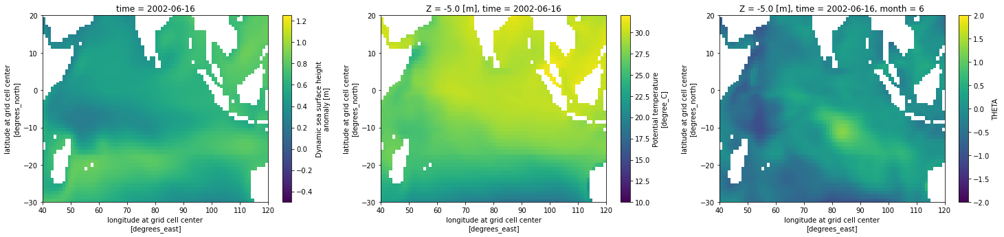
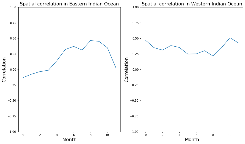
Perform the correlations in the east and west Indian Ocean

# Western and Eastern Indian Ocean regions (WIO and EIO respectively)
# EIO; 90 –110 E, 10 S–0N
# WIO; 50 –70 E, 10 S–10 N

# Group Eastern Indian Ocean  data by month. This will make the correlation of all monthly values straightforwrd.
ssh_group = ssh_ds_masked['SSH'].sel(longitude=slice(90,110),latitude=slice(-10,0)).groupby('time.month')
#temp_group = temp_ds_masked['THETA'].sel(longitude=slice(90,110),latitude=slice(-10,0), Z=-5.0).drop('Z').groupby('time.month')
temp_group = temp_ds_masked_anomaly['THETA'].sel(longitude=slice(90,110),latitude=slice(-10,0), Z=-5.0).drop('Z').groupby('time.month')

print(" Running correlations in eastern Indian Ocean . . .\n")  
corr = []
for month in range(1,13):
    corr.append(xr.corr(ssh_group[month], temp_group[month]))
    #print("\nthe correlation in the east is: " , xr.corr(ssh_group[month], temp_group[month]).values)
    
# Do some plotting
fig,ax=plt.subplots(1,2,figsize=(14,8))

ax[0].set_title("Spatial correlation in Eastern Indian Ocean",fontsize=16)
ax[0].set_ylabel("Correlation",fontsize=16)
ax[0].set_xlabel("Month",fontsize=16)
ax[0].set_ylim([-1, 1])
ax[0].plot(corr)

# Repeat for Western Indian Ocean
# Group the data by month. This will make the correlation of all monthly values straightforwrd.
ssh_group = ssh_ds_masked['SSH'].sel(longitude=slice(50,70),latitude=slice(-10,10)).groupby('time.month')
#temp_group = temp_ds_masked['THETA'].sel(longitude=slice(50,70),latitude=slice(-10,10), Z=-5.0).drop('Z').groupby('time.month')
temp_group = temp_ds_masked_anomaly['THETA'].sel(longitude=slice(50,70),latitude=slice(-10,10), Z=-5.0).drop('Z').groupby('time.month')


print(" Running correlations in western Indian Ocean . . .\n") 
corr2 =[]
for month in range(1,13):
    corr2.append(xr.corr(ssh_group[month], temp_group[month]))
    #print("\nthe correlation in the west is: " , xr.corr(ssh_group[month], temp_group[month]).values)
    
ax[1].set_title("Spatial correlation in Western Indian Ocean",fontsize=16)
ax[1].set_ylabel("Correlation",fontsize=16)
ax[1].set_xlabel("Month",fontsize=16)
ax[1].set_ylim([-1, 1])
ax[1].plot(corr2)

 Running correlations in eastern Indian Ocean . . .

 Running correlations in western Indian Ocean . . .

End