From the PO.DAAC Cookbook, to access the GitHub version of the notebook, follow this link.

MUR Sea Surface Temperature Analysis of Washington State

Requirement:

  1. Compute environment

This tutorial can only be run in an AWS cloud instance running in us-west-2: NASA Earthdata Cloud data in S3 can be directly accessed via temporary credentials; this access is limited to requests made within the US West (Oregon) (code: us-west-2) AWS region.

  1. Earthdata Login

An Earthdata Login account is required to access data, as well as discover restricted data, from the NASA Earthdata system. Thus, to access NASA data, you need Earthdata Login. Please visit https://urs.earthdata.nasa.gov to register and manage your Earthdata Login account. This account is free to create and only takes a moment to set up.

Learning Objectives:

  • Access cloud-stored MUR Global SST data within AWS cloud, without downloading it to your local machine
  • Visualize and analyze data in a use case example
  • Use earthaccess library to search for, access, and download the data

GHRSST Level 4 MUR Global Foundation Sea Surface Temperature Analysis (v4.1) Dataset:

  1. MUR-JPL-L4-GLOB-v4.1

DOI: https://doi.org/10.5067/GHGMR-4FJ04

Notebook Author: Zoë Walschots, NASA PO.DAAC (Aug 2023)

Import Packages

import h5netcdf
import xarray as xr
import numpy as np
import matplotlib.pyplot as plt
import hvplot.xarray
import cartopy.crs as ccrs
import cartopy.feature as cfeat
import earthaccess
from earthaccess import Auth, DataCollections, DataGranules, Store

In this notebook, we will be calling the authentication in the below cell.

auth = earthaccess.login(strategy="interactive", persist=True)

Access and Visualize Data

Let’s look at the Sea Surface Temperature of first summer we have data for (2012) using earthaccess

mur_results = earthaccess.search_data(short_name = 'MUR-JPL-L4-GLOB-v4.1', temporal = ('2012-05-21', '2012-08-20'), bounding_box = ('-125.41992','45.61181','-116.64844','49.2315'))
Granules found: 92
ds_mur = xr.open_mfdataset(earthaccess.open(mur_results), engine = 'h5netcdf')
ds_mur
 Opening 92 granules, approx size: 0.0 GB
<xarray.Dataset>
Dimensions:           (time: 92, lat: 17999, lon: 36000)
Coordinates:
  * time              (time) datetime64[ns] 2012-05-21T09:00:00 ... 2012-08-2...
  * lat               (lat) float32 -89.99 -89.98 -89.97 ... 89.97 89.98 89.99
  * lon               (lon) float32 -180.0 -180.0 -180.0 ... 180.0 180.0 180.0
Data variables:
    analysed_sst      (time, lat, lon) float32 dask.array<chunksize=(1, 17999, 36000), meta=np.ndarray>
    analysis_error    (time, lat, lon) float32 dask.array<chunksize=(1, 17999, 36000), meta=np.ndarray>
    mask              (time, lat, lon) float32 dask.array<chunksize=(1, 17999, 36000), meta=np.ndarray>
    sea_ice_fraction  (time, lat, lon) float32 dask.array<chunksize=(1, 17999, 36000), meta=np.ndarray>
Attributes: (12/47)
    Conventions:                CF-1.5
    title:                      Daily MUR SST, Final product
    summary:                    A merged, multi-sensor L4 Foundation SST anal...
    references:                 http://podaac.jpl.nasa.gov/Multi-scale_Ultra-...
    institution:                Jet Propulsion Laboratory
    history:                    created at nominal 4-day latency; replaced nr...
    ...                         ...
    project:                    NASA Making Earth Science Data Records for Us...
    publisher_name:             GHRSST Project Office
    publisher_url:              http://www.ghrsst.org
    publisher_email:            ghrsst-po@nceo.ac.uk
    processing_level:           L4
    cdm_data_type:              grid
    • time
      PandasIndex
      PandasIndex(DatetimeIndex(['2012-05-21 09:00:00', '2012-05-22 09:00:00',
                     '2012-05-23 09:00:00', '2012-05-24 09:00:00',
                     '2012-05-25 09:00:00', '2012-05-26 09:00:00',
                     '2012-05-27 09:00:00', '2012-05-28 09:00:00',
                     '2012-05-29 09:00:00', '2012-05-30 09:00:00',
                     '2012-05-31 09:00:00', '2012-06-01 09:00:00',
                     '2012-06-02 09:00:00', '2012-06-03 09:00:00',
                     '2012-06-04 09:00:00', '2012-06-05 09:00:00',
                     '2012-06-06 09:00:00', '2012-06-07 09:00:00',
                     '2012-06-08 09:00:00', '2012-06-09 09:00:00',
                     '2012-06-10 09:00:00', '2012-06-11 09:00:00',
                     '2012-06-12 09:00:00', '2012-06-13 09:00:00',
                     '2012-06-14 09:00:00', '2012-06-15 09:00:00',
                     '2012-06-16 09:00:00', '2012-06-17 09:00:00',
                     '2012-06-18 09:00:00', '2012-06-19 09:00:00',
                     '2012-06-20 09:00:00', '2012-06-21 09:00:00',
                     '2012-06-22 09:00:00', '2012-06-23 09:00:00',
                     '2012-06-24 09:00:00', '2012-06-25 09:00:00',
                     '2012-06-26 09:00:00', '2012-06-27 09:00:00',
                     '2012-06-28 09:00:00', '2012-06-29 09:00:00',
                     '2012-06-30 09:00:00', '2012-07-01 09:00:00',
                     '2012-07-02 09:00:00', '2012-07-03 09:00:00',
                     '2012-07-04 09:00:00', '2012-07-05 09:00:00',
                     '2012-07-06 09:00:00', '2012-07-07 09:00:00',
                     '2012-07-08 09:00:00', '2012-07-09 09:00:00',
                     '2012-07-10 09:00:00', '2012-07-11 09:00:00',
                     '2012-07-12 09:00:00', '2012-07-13 09:00:00',
                     '2012-07-14 09:00:00', '2012-07-15 09:00:00',
                     '2012-07-16 09:00:00', '2012-07-17 09:00:00',
                     '2012-07-18 09:00:00', '2012-07-19 09:00:00',
                     '2012-07-20 09:00:00', '2012-07-21 09:00:00',
                     '2012-07-22 09:00:00', '2012-07-23 09:00:00',
                     '2012-07-24 09:00:00', '2012-07-25 09:00:00',
                     '2012-07-26 09:00:00', '2012-07-27 09:00:00',
                     '2012-07-28 09:00:00', '2012-07-29 09:00:00',
                     '2012-07-30 09:00:00', '2012-07-31 09:00:00',
                     '2012-08-01 09:00:00', '2012-08-02 09:00:00',
                     '2012-08-03 09:00:00', '2012-08-04 09:00:00',
                     '2012-08-05 09:00:00', '2012-08-06 09:00:00',
                     '2012-08-07 09:00:00', '2012-08-08 09:00:00',
                     '2012-08-09 09:00:00', '2012-08-10 09:00:00',
                     '2012-08-11 09:00:00', '2012-08-12 09:00:00',
                     '2012-08-13 09:00:00', '2012-08-14 09:00:00',
                     '2012-08-15 09:00:00', '2012-08-16 09:00:00',
                     '2012-08-17 09:00:00', '2012-08-18 09:00:00',
                     '2012-08-19 09:00:00', '2012-08-20 09:00:00'],
                    dtype='datetime64[ns]', name='time', freq=None))
    • lat
      PandasIndex
      PandasIndex(Index([-89.98999786376953,  -89.9800033569336, -89.97000122070312,
             -89.95999908447266, -89.94999694824219, -89.94000244140625,
             -89.93000030517578, -89.91999816894531, -89.91000366210938,
              -89.9000015258789,
             ...
               89.9000015258789,  89.91000366210938,  89.91999816894531,
              89.93000030517578,  89.94000244140625,  89.94999694824219,
              89.95999908447266,  89.97000122070312,   89.9800033569336,
              89.98999786376953],
            dtype='float32', name='lat', length=17999))
    • lon
      PandasIndex
      PandasIndex(Index([-179.99000549316406, -179.97999572753906, -179.97000122070312,
              -179.9600067138672,  -179.9499969482422, -179.94000244140625,
             -179.92999267578125,  -179.9199981689453, -179.91000366210938,
             -179.89999389648438,
             ...
              179.91000366210938,   179.9199981689453,  179.92999267578125,
              179.94000244140625,   179.9499969482422,   179.9600067138672,
              179.97000122070312,  179.97999572753906,  179.99000549316406,
                           180.0],
            dtype='float32', name='lon', length=36000))
  • Conventions :
    CF-1.5
    title :
    Daily MUR SST, Final product
    summary :
    A merged, multi-sensor L4 Foundation SST analysis product from JPL.
    references :
    http://podaac.jpl.nasa.gov/Multi-scale_Ultra-high_Resolution_MUR-SST
    institution :
    Jet Propulsion Laboratory
    history :
    created at nominal 4-day latency; replaced nrt (1-day latency) version.
    comment :
    MUR = "Multi-scale Ultra-high Reolution"
    license :
    These data are available free of charge under data policy of JPL PO.DAAC.
    id :
    MUR-JPL-L4-GLOB-v04.1
    naming_authority :
    org.ghrsst
    product_version :
    04.1
    uuid :
    27665bc0-d5fc-11e1-9b23-0800200c9a66
    gds_version_id :
    2.0
    netcdf_version_id :
    4.1
    date_created :
    20150711T060041Z
    start_time :
    20120521T090000Z
    stop_time :
    20120521T090000Z
    time_coverage_start :
    20120520T210000Z
    time_coverage_end :
    20120521T210000Z
    file_quality_level :
    1
    source :
    AVHRR18_G-NAVO, AVHRR19_G-NAVO, AVHRR_METOP_A-EUMETSAT, MODIS_A-JPL, MODIS_T-JPL, WSAT-REMSS, iQUAM-NOAA/NESDIS, Ice_Conc-OSISAF
    platform :
    Aqua, DMSP, NOAA-POES, Suomi-NPP, Terra
    sensor :
    AMSR-E, AVHRR, MODIS, SSM/I, VIIRS, in-situ
    Metadata_Conventions :
    Unidata Observation Dataset v1.0
    metadata_link :
    http://podaac.jpl.nasa.gov/ws/metadata/dataset/?format=iso&shortName=MUR-JPL-L4-GLOB-v04.1
    keywords :
    Oceans > Ocean Temperature > Sea Surface Temperature
    keywords_vocabulary :
    NASA Global Change Master Directory (GCMD) Science Keywords
    standard_name_vocabulary :
    NetCDF Climate and Forecast (CF) Metadata Convention
    southernmost_latitude :
    -90.0
    northernmost_latitude :
    90.0
    westernmost_longitude :
    -180.0
    easternmost_longitude :
    180.0
    spatial_resolution :
    0.01 degrees
    geospatial_lat_units :
    degrees north
    geospatial_lat_resolution :
    0.01 degrees
    geospatial_lon_units :
    degrees east
    geospatial_lon_resolution :
    0.01 degrees
    acknowledgment :
    Please acknowledge the use of these data with the following statement: These data were provided by JPL under support by NASA MEaSUREs program.
    creator_name :
    JPL MUR SST project
    creator_email :
    ghrsst@podaac.jpl.nasa.gov
    creator_url :
    http://mur.jpl.nasa.gov
    project :
    NASA Making Earth Science Data Records for Use in Research Environments (MEaSUREs) Program
    publisher_name :
    GHRSST Project Office
    publisher_url :
    http://www.ghrsst.org
    publisher_email :
    ghrsst-po@nceo.ac.uk
    processing_level :
    L4
    cdm_data_type :
    grid
  • # we want the sea surface temperature variable for this visualization
    ds = ds_mur['analysed_sst']
    
    # Subset the dataset so that the program can run the code better
    ds_subset = ds.sel(time=slice('2012-05-21T09:00:00', '2012-08-20T09:00:00'))
    lat_range = slice(45.61181, 49.2315)
    lon_range = slice(-125.41992, -116.64844)
    ds_subset = ds_subset.sel(lat=lat_range, lon=lon_range)

    To plot the data, we will be looking at the mean temperature across the summer.

    # Calculate the mean across the time dimension
    mean_data = ds_subset.mean(dim='time')
    #plot the figure
    fig = plt.figure(figsize=(12, 6))
    ax = plt.axes(projection=ccrs.PlateCarree())
    
    colorbar_range = (282, 291)
    
    im = ax.imshow(mean_data.values, cmap='YlOrRd', origin='lower', transform=ccrs.PlateCarree(),
                   extent=[mean_data.lon.min(), mean_data.lon.max(), mean_data.lat.min(), mean_data.lat.max()])
    
    im.set_clim(vmin=colorbar_range[0], vmax=colorbar_range[1])
    cbar = plt.colorbar(im, ax=ax, orientation='horizontal', pad=0.05, shrink=0.7)
    cbar.set_label('Sea Surface Temperature (Kelvin)')
    ax.set_title('Mean Sea Surface Temperature Summer 2012') 
    ax.coastlines()
    ax.gridlines()
    
    plt.show()

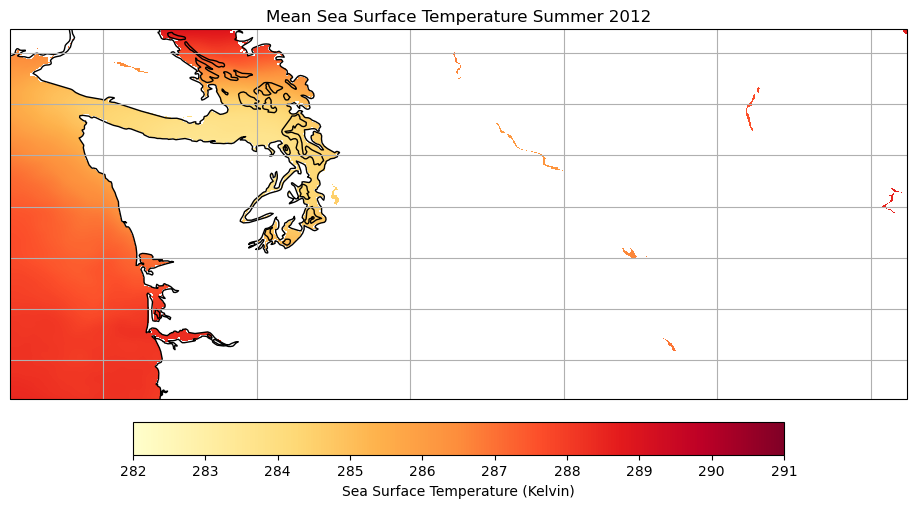
    Let’s also look at the most recent summer we have data for (2022) in comparison.

    mur_results_2 = earthaccess.search_data(short_name = 'MUR-JPL-L4-GLOB-v4.1', temporal = ('2022-05-21', '2022-08-20'), bounding_box = ('-125.41992','45.61181','-116.64844','49.2315'))
    Granules found: 92
    ds_mur_2 = xr.open_mfdataset(earthaccess.open(mur_results_2), engine = 'h5netcdf')
    ds_mur_2
     Opening 92 granules, approx size: 0.0 GB
    <xarray.Dataset>
    Dimensions:           (time: 92, lat: 17999, lon: 36000)
    Coordinates:
      * time              (time) datetime64[ns] 2022-05-21T09:00:00 ... 2022-08-2...
      * lat               (lat) float32 -89.99 -89.98 -89.97 ... 89.97 89.98 89.99
      * lon               (lon) float32 -180.0 -180.0 -180.0 ... 180.0 180.0 180.0
    Data variables:
        analysed_sst      (time, lat, lon) float32 dask.array<chunksize=(1, 17999, 36000), meta=np.ndarray>
        analysis_error    (time, lat, lon) float32 dask.array<chunksize=(1, 17999, 36000), meta=np.ndarray>
        mask              (time, lat, lon) float32 dask.array<chunksize=(1, 17999, 36000), meta=np.ndarray>
        sea_ice_fraction  (time, lat, lon) float32 dask.array<chunksize=(1, 17999, 36000), meta=np.ndarray>
        dt_1km_data       (time, lat, lon) timedelta64[ns] dask.array<chunksize=(1, 17999, 36000), meta=np.ndarray>
        sst_anomaly       (time, lat, lon) float32 dask.array<chunksize=(1, 17999, 36000), meta=np.ndarray>
    Attributes: (12/47)
        Conventions:                CF-1.7
        title:                      Daily MUR SST, Final product
        summary:                    A merged, multi-sensor L4 Foundation SST anal...
        references:                 http://podaac.jpl.nasa.gov/Multi-scale_Ultra-...
        institution:                Jet Propulsion Laboratory
        history:                    created at nominal 4-day latency; replaced nr...
        ...                         ...
        project:                    NASA Making Earth Science Data Records for Us...
        publisher_name:             GHRSST Project Office
        publisher_url:              http://www.ghrsst.org
        publisher_email:            ghrsst-po@nceo.ac.uk
        processing_level:           L4
        cdm_data_type:              grid
    • time
      PandasIndex
      PandasIndex(DatetimeIndex(['2022-05-21 09:00:00', '2022-05-22 09:00:00',
                     '2022-05-23 09:00:00', '2022-05-24 09:00:00',
                     '2022-05-25 09:00:00', '2022-05-26 09:00:00',
                     '2022-05-27 09:00:00', '2022-05-28 09:00:00',
                     '2022-05-29 09:00:00', '2022-05-30 09:00:00',
                     '2022-05-31 09:00:00', '2022-06-01 09:00:00',
                     '2022-06-02 09:00:00', '2022-06-03 09:00:00',
                     '2022-06-04 09:00:00', '2022-06-05 09:00:00',
                     '2022-06-06 09:00:00', '2022-06-07 09:00:00',
                     '2022-06-08 09:00:00', '2022-06-09 09:00:00',
                     '2022-06-10 09:00:00', '2022-06-11 09:00:00',
                     '2022-06-12 09:00:00', '2022-06-13 09:00:00',
                     '2022-06-14 09:00:00', '2022-06-15 09:00:00',
                     '2022-06-16 09:00:00', '2022-06-17 09:00:00',
                     '2022-06-18 09:00:00', '2022-06-19 09:00:00',
                     '2022-06-20 09:00:00', '2022-06-21 09:00:00',
                     '2022-06-22 09:00:00', '2022-06-23 09:00:00',
                     '2022-06-24 09:00:00', '2022-06-25 09:00:00',
                     '2022-06-26 09:00:00', '2022-06-27 09:00:00',
                     '2022-06-28 09:00:00', '2022-06-29 09:00:00',
                     '2022-06-30 09:00:00', '2022-07-01 09:00:00',
                     '2022-07-02 09:00:00', '2022-07-03 09:00:00',
                     '2022-07-04 09:00:00', '2022-07-05 09:00:00',
                     '2022-07-06 09:00:00', '2022-07-07 09:00:00',
                     '2022-07-08 09:00:00', '2022-07-09 09:00:00',
                     '2022-07-10 09:00:00', '2022-07-11 09:00:00',
                     '2022-07-12 09:00:00', '2022-07-13 09:00:00',
                     '2022-07-14 09:00:00', '2022-07-15 09:00:00',
                     '2022-07-16 09:00:00', '2022-07-17 09:00:00',
                     '2022-07-18 09:00:00', '2022-07-19 09:00:00',
                     '2022-07-20 09:00:00', '2022-07-21 09:00:00',
                     '2022-07-22 09:00:00', '2022-07-23 09:00:00',
                     '2022-07-24 09:00:00', '2022-07-25 09:00:00',
                     '2022-07-26 09:00:00', '2022-07-27 09:00:00',
                     '2022-07-28 09:00:00', '2022-07-29 09:00:00',
                     '2022-07-30 09:00:00', '2022-07-31 09:00:00',
                     '2022-08-01 09:00:00', '2022-08-02 09:00:00',
                     '2022-08-03 09:00:00', '2022-08-04 09:00:00',
                     '2022-08-05 09:00:00', '2022-08-06 09:00:00',
                     '2022-08-07 09:00:00', '2022-08-08 09:00:00',
                     '2022-08-09 09:00:00', '2022-08-10 09:00:00',
                     '2022-08-11 09:00:00', '2022-08-12 09:00:00',
                     '2022-08-13 09:00:00', '2022-08-14 09:00:00',
                     '2022-08-15 09:00:00', '2022-08-16 09:00:00',
                     '2022-08-17 09:00:00', '2022-08-18 09:00:00',
                     '2022-08-19 09:00:00', '2022-08-20 09:00:00'],
                    dtype='datetime64[ns]', name='time', freq=None))
    • lat
      PandasIndex
      PandasIndex(Index([-89.98999786376953,  -89.9800033569336, -89.97000122070312,
             -89.95999908447266, -89.94999694824219, -89.94000244140625,
             -89.93000030517578, -89.91999816894531, -89.91000366210938,
              -89.9000015258789,
             ...
               89.9000015258789,  89.91000366210938,  89.91999816894531,
              89.93000030517578,  89.94000244140625,  89.94999694824219,
              89.95999908447266,  89.97000122070312,   89.9800033569336,
              89.98999786376953],
            dtype='float32', name='lat', length=17999))
    • lon
      PandasIndex
      PandasIndex(Index([-179.99000549316406, -179.97999572753906, -179.97000122070312,
              -179.9600067138672,  -179.9499969482422, -179.94000244140625,
             -179.92999267578125,  -179.9199981689453, -179.91000366210938,
             -179.89999389648438,
             ...
              179.91000366210938,   179.9199981689453,  179.92999267578125,
              179.94000244140625,   179.9499969482422,   179.9600067138672,
              179.97000122070312,  179.97999572753906,  179.99000549316406,
                           180.0],
            dtype='float32', name='lon', length=36000))
  • Conventions :
    CF-1.7
    title :
    Daily MUR SST, Final product
    summary :
    A merged, multi-sensor L4 Foundation SST analysis product from JPL.
    references :
    http://podaac.jpl.nasa.gov/Multi-scale_Ultra-high_Resolution_MUR-SST
    institution :
    Jet Propulsion Laboratory
    history :
    created at nominal 4-day latency; replaced nrt (1-day latency) version.
    comment :
    MUR = "Multi-scale Ultra-high Resolution"
    license :
    These data are available free of charge under data policy of JPL PO.DAAC.
    id :
    MUR-JPL-L4-GLOB-v04.1
    naming_authority :
    org.ghrsst
    product_version :
    04.1
    uuid :
    27665bc0-d5fc-11e1-9b23-0800200c9a66
    gds_version_id :
    2.0
    netcdf_version_id :
    4.1
    date_created :
    20220530T072023Z
    start_time :
    20220521T090000Z
    stop_time :
    20220521T090000Z
    time_coverage_start :
    20220520T210000Z
    time_coverage_end :
    20220521T210000Z
    file_quality_level :
    3
    source :
    MODIS_T-JPL, MODIS_A-JPL, AMSR2-REMSS, AVHRRMTB_G-NAVO, iQUAM-NOAA/NESDIS, Ice_Conc-OSISAF
    platform :
    Terra, Aqua, GCOM-W, MetOp-B, Buoys/Ships
    sensor :
    MODIS, AMSR2, AVHRR, in-situ
    Metadata_Conventions :
    Unidata Observation Dataset v1.0
    metadata_link :
    http://podaac.jpl.nasa.gov/ws/metadata/dataset/?format=iso&shortName=MUR-JPL-L4-GLOB-v04.1
    keywords :
    Oceans > Ocean Temperature > Sea Surface Temperature
    keywords_vocabulary :
    NASA Global Change Master Directory (GCMD) Science Keywords
    standard_name_vocabulary :
    NetCDF Climate and Forecast (CF) Metadata Convention
    southernmost_latitude :
    -90.0
    northernmost_latitude :
    90.0
    westernmost_longitude :
    -180.0
    easternmost_longitude :
    180.0
    spatial_resolution :
    0.01 degrees
    geospatial_lat_units :
    degrees north
    geospatial_lat_resolution :
    0.01
    geospatial_lon_units :
    degrees east
    geospatial_lon_resolution :
    0.01
    acknowledgment :
    Please acknowledge the use of these data with the following statement: These data were provided by JPL under support by NASA MEaSUREs program.
    creator_name :
    JPL MUR SST project
    creator_email :
    ghrsst@podaac.jpl.nasa.gov
    creator_url :
    http://mur.jpl.nasa.gov
    project :
    NASA Making Earth Science Data Records for Use in Research Environments (MEaSUREs) Program
    publisher_name :
    GHRSST Project Office
    publisher_url :
    http://www.ghrsst.org
    publisher_email :
    ghrsst-po@nceo.ac.uk
    processing_level :
    L4
    cdm_data_type :
    grid
  • ds_2 = ds_mur_2['analysed_sst']
    
    ds_subset_2 = ds_2.sel(time=slice('2022-05-21T09:00:00', '2022-08-20T09:00:00'))
    ds_subset_2 = ds_subset_2.sel(lat=lat_range, lon=lon_range)
    mean_data_2 = ds_subset_2.mean(dim='time')
    fig = plt.figure(figsize=(12, 6))
    ax = plt.axes(projection=ccrs.PlateCarree())
    colorbar_range = (282, 291)
    
    im = ax.imshow(mean_data_2.values, cmap='YlOrRd', origin='lower', transform=ccrs.PlateCarree(),
                   extent=[mean_data_2.lon.min(), mean_data_2.lon.max(), mean_data_2.lat.min(), mean_data_2.lat.max()])
    
    im.set_clim(vmin=colorbar_range[0], vmax=colorbar_range[1])
    cbar = plt.colorbar(im, ax=ax, orientation='horizontal', pad=0.05, shrink=0.7)
    cbar.set_label('Sea Surface Temperature (Kelvin)') 
    ax.set_title('Mean Sea Surface Temperature Summer 2022')
    ax.coastlines()
    ax.gridlines()
    
    plt.show()

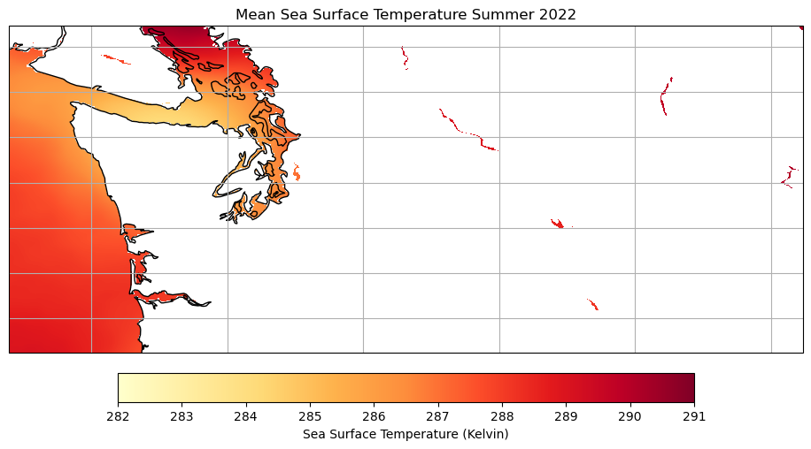
    Let’s plot the difference between these two summers.

    # Calculate the difference between the two mean datasets
    data_diff = mean_data_2 - mean_data
    fig = plt.figure(figsize=(12, 6))
    ax = plt.axes(projection=ccrs.PlateCarree())
    
    colorbar_range = (-3, 3)
    
    im = ax.imshow(data_diff.values, cmap='coolwarm', origin='lower', transform=ccrs.PlateCarree(),
                   extent=[mean_data.lon.min(), mean_data.lon.max(), mean_data.lat.min(), mean_data.lat.max()],
                   vmin=colorbar_range[0], vmax=colorbar_range[1]) 
    
    cbar = plt.colorbar(im, ax=ax, orientation='horizontal', pad=0.05, shrink=0.7)
    cbar.set_label('Sea Surface Temperature Difference (Kelvin)')
    ax.set_title('Sea Surface Temperature Difference (Avg of Summer 2022 - Avg of Summer 2012)')
    
    ax.coastlines()
    ax.gridlines()
    
    plt.show()

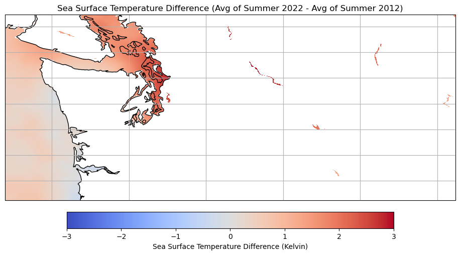
    Let’s zoom in on Lake Chelan in central Washington to look at the difference between the averages of the two summers.

    #subset the data for Lake Chelan in 2012
    ds_subset_3 = ds.sel(time=slice('2012-05-21T09:00:00', '2012-08-20T09:00:00'))
    lat_range_2 = slice(47.7926, 48.44274)
    lon_range_2 = slice(-120.99902, -119.77734)
    ds_subset_3 = ds_subset_3.sel(lat=lat_range_2, lon=lon_range_2)
    
    mean_data_3 = ds_subset_3.mean(dim='time')
    #subset the data for Lake Chelan in 2022
    ds_subset_4 = ds_2.sel(time=slice('2022-05-21T09:00:00', '2022-08-20T09:00:00'))
    ds_subset_4 = ds_subset_4.sel(lat=lat_range_2, lon=lon_range_2)
    
    mean_data_4 = ds_subset_4.mean(dim='time')
    # Calculate the difference between the two mean datasets
    data_diff_2 = mean_data_4 - mean_data_3
    fig = plt.figure(figsize=(12, 6))
    ax = plt.axes(projection=ccrs.PlateCarree())
    
    colorbar_range = (2, 3.5)
    
    im = ax.imshow(data_diff_2.values, cmap='YlOrRd', origin='lower', transform=ccrs.PlateCarree(),
                   extent=[data_diff_2.lon.min(), data_diff_2.lon.max(), data_diff_2.lat.min(), data_diff_2.lat.max()])
    
    im.set_clim(vmin=colorbar_range[0], vmax=colorbar_range[1])
    cbar = plt.colorbar(im, ax=ax, orientation='horizontal', pad=0.05, shrink=0.7)
    cbar.set_label('Sea Surface Temperature Difference (Kelvin)')
    ax.set_title('Lake Chelan Sea Surface Temperature Difference 2012 vs 2022')
    
    ax.gridlines()
    
    plt.show()

    Please note that the GHRSST dataset is optimized for ocean sea surface temperature, so caution should be exercised when visualizing inland water bodies.