From the PO.DAAC Cookbook, to access the GitHub version of the notebook, follow this link.

Scale Scientific Analysis in the Cloud with AWS Lambda

This tutorial demonstrates how to invoke an AWS Lambda function to create a timeseries of global mean sea surface temperature values.

IMPORTANT: This notebook will only run successfully after deploying the AWS Lambda function and supporting services to your own Amazon Web Services account.

See the full documentation to set up the prerequisite services.

** Note that using AWS Compute services will incur costs that will be charged to your AWS account. Running this tutorial as-configured with no modifications should result in less than $1 USD of charges. Expanding the analysis to a longer time period or different dataset will affect the compute costs charged to your AWS account.

PO.DAAC is not responsible for costs charged as a result of running this tutorial

Prerequisite Steps: Set up AWS infrastructure

This tutorial takes advantage of numerous AWS Services including Lambda, Parameter Store, Elastic Compute Cloud (EC2), Elastic Container Registry (ECR), and Simple Storage Service (S3).

After setting up and deploying all of the services as described in the documentation, this notebook must be run in an EC2 instance to invoke the functions and plot the results.

Connect to EC2 instance to run this notebook

This notebook cannot be run on a local computer, as it heavily depends on direct in-cloud access. To run this notebook in AWS, connect to an EC2 instance running in the us-west-2 region, following the instructions in this tutorial. Once you have connected to the EC2 instance, you can clone this repository into that environment, install the required packages, and run this notebook.

Step 1: Log in to Earthdata

We use the earthaccess Python library to handle Earthdata authentication for the initial query to find the granules of interest.

import earthaccess
import json
import boto3
import s3fs
import xarray as xr
import matplotlib as mpl
import matplotlib.pyplot as plt

auth = earthaccess.login()

EARTHDATA_USERNAME and EARTHDATA_PASSWORD are not set in the current environment, try setting them or use a different strategy (netrc, interactive)
You're now authenticated with NASA Earthdata Login
Using token with expiration date: 06/16/2023
Using .netrc file for EDL

granules = earthaccess.search_data(
    short_name='MUR25-JPL-L4-GLOB-v04.2',
    cloud_hosted=True,
    temporal=("2022-01-01", "2023-01-01")
)

Granules found: 365

granule_paths = [g.data_links(access='direct')[0] for g in granules]

for path in granule_paths:
    print(path)
    break

s3://podaac-ops-cumulus-protected/MUR25-JPL-L4-GLOB-v04.2/20220101090000-JPL-L4_GHRSST-SSTfnd-MUR25-GLOB-v02.0-fv04.2.nc

Step 2: Invoke the Lambda function

Set up a boto3 session to connect to your AWS instance and invoke the Lambda function

session = boto3.Session(profile_name='saml-pub')

lambda_client = session.client('lambda', region_name='us-west-2')

s3_results_bucket = "podaac-sst"

for granule in granule_paths:
    lambda_payload = {"input_granule_s3path": granule, "output_granule_s3bucket": s3_results_bucket, "prefix":"podaac"}

    lambda_client.invoke(
        FunctionName="podaac-sst",
        InvocationType="Event",
        Payload=json.dumps(lambda_payload)
    )

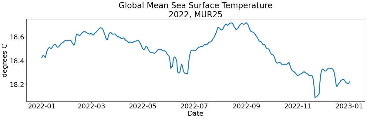
Step 3: Plot results as timeseries

Open the resulting global mean files in xarray:

# set up the connection to the S3 bucket holding the results
s3_results = s3fs.S3FileSystem(
    anon=False,
    profile='saml-pub'
)

s3_files = s3_results.glob("s3://" + s3_results_bucket + "/MUR25/*")


# iterate through s3 files to create a fileset
fileset = [s3_results.open(file) for file in s3_files]

# open all files as an xarray dataset
data = xr.open_mfdataset(fileset, combine='by_coords', engine='scipy')

data

<xarray.Dataset>
Dimensions:       (time: 365)
Coordinates:
  * time          (time) datetime64[ns] 2022-01-01T09:00:00 ... 2023-01-01T09...
Data variables:
    analysed_sst  (time) float64 dask.array<chunksize=(1,), meta=np.ndarray>

xarray.Dataset

• Dimensions:
  • time: 365
• Coordinates: (1)
  • time
    (time)
    datetime64[ns]
    2022-01-01T09:00:00 ... 2023-01-...

    array(['2022-01-01T09:00:00.000000000', '2022-01-02T09:00:00.000000000',
           '2022-01-03T09:00:00.000000000', ..., '2022-12-30T09:00:00.000000000',
           '2022-12-31T09:00:00.000000000', '2023-01-01T09:00:00.000000000'],
          dtype='datetime64[ns]')

• Data variables: (1)
  • analysed_sst
    (time)
    float64
    dask.array<chunksize=(1,), meta=np.ndarray>

    description :

    Area-weighted global mean sea surface temperature calculated using AWS Lambda

    units :

    celcius

    date_created :

    Jun-06-2023

    Array Chunk Bytes 2.85 kiB 8 B Shape (365,) (1,) Dask graph 365 chunks in 731 graph layers Data type float64 numpy.ndarray

• Indexes: (1)
  • time
    PandasIndex

    PandasIndex(DatetimeIndex(['2022-01-01 09:00:00', '2022-01-02 09:00:00',
                   '2022-01-03 09:00:00', '2022-01-04 09:00:00',
                   '2022-01-05 09:00:00', '2022-01-06 09:00:00',
                   '2022-01-07 09:00:00', '2022-01-08 09:00:00',
                   '2022-01-09 09:00:00', '2022-01-10 09:00:00',
                   ...
                   '2022-12-23 09:00:00', '2022-12-24 09:00:00',
                   '2022-12-25 09:00:00', '2022-12-26 09:00:00',
                   '2022-12-27 09:00:00', '2022-12-28 09:00:00',
                   '2022-12-29 09:00:00', '2022-12-30 09:00:00',
                   '2022-12-31 09:00:00', '2023-01-01 09:00:00'],
                  dtype='datetime64[ns]', name='time', length=365, freq=None))

• Attributes: (0)

Plot the data using matplotlib:

mpl.rcParams.update({'font.size': 22})

# set up the figure
fig = plt.Figure(figsize=(20,5))

# plot the data
plt.plot(data.time, data.analysed_sst, linewidth='3')
plt.title('Global Mean Sea Surface Temperature' + '\n' + '2022, MUR25')

plt.ylabel('degrees C')
plt.xlabel('Date')

Text(0.5, 0, 'Date')