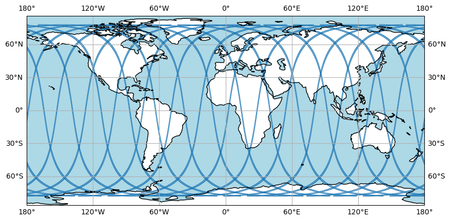
cycle_number: One cycle represents when SWOT covers approximate global coverage (21 days of data)
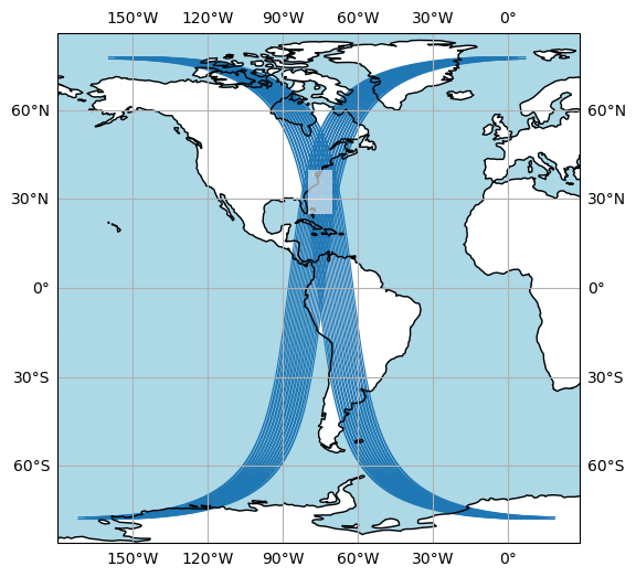
pass_number: One swath represents one pass. Each granule/file in PO.DAAC is exactly one SWOT pass. The same pass number across cycles should match up spatially
num_lines and num_pixels represent the “length” and “width” of a satellite swath
num_sides represents the two swaths that the SWOT KaRIn instrument records. Here is an excellent visual.
Here, we use a JSON file of the entire dataset made using Kerchunk for efficiently processing large amounts of data in the cloud
We read in the file as zarr cloud-optimized data store from the chunked JSON
Read JSON from VEDA and save locally
veda = s3fs.S3FileSystem()with veda.open("s3://veda-data-store-staging/SWOT_L2_LR_SSH_2.0/SWOT_L2_LR_SSH_Expert_2.0.json", 'r') as infile:withopen("SWOT_L2_LR_SSH_Expert_2.0.json", 'w') as outfile: ujson.dump(ujson.load(infile), outfile)
Model estimate of the effect on sea surface topography due to high frequency air pressure and wind effects and the low-frequency height from inverted barometer effect (inv_bar_cor). This value is subtracted from the ssh_karin and ssh_karin_2 to compute ssha_karin and ssha_karin_2, respectively. Use only one of inv_bar_cor and dac.
Geoid height above the reference ellipsoid with a correction to refer the value to the mean tide system, i.e. includes the permanent tide (zero frequency).
Height correction from crossover calibration. To apply this correction the value of height_cor_xover should be added to the value of ssh_karin, ssh_karin_2, ssha_karin, and ssha_karin_2.
Flag indicating the quality of the height correction from crossover calibration. Values of 0, 1, and 2 indicate that the correction is good, suspect, and bad, respectively.
flag_meanings :
good suspect bad
flag_values :
[0, 1, 2]
long_name :
quality flag for height correction from crossover calibration
Estimate of static effect of atmospheric pressure on sea surface height. Above average pressure lowers sea surface height. Computed by interpolating ECMWF pressure fields in space and time. The value is included in dac. To apply, add dac to ssha_karin and ssha_karin_2 and subtract inv_bar_cor.
long_name :
static inverse barometer effect on sea surface height
Equivalent vertical correction due to ionosphere delay. The reported sea surface height, latitude and longitude are computed after adding negative media corrections to uncorrected range along slant-range paths, accounting for the differential delay between the two KaRIn antennas. The equivalent vertical correction is computed by applying obliquity factors to the slant-path correction. Adding the reported correction to the reported sea surface height results in the uncorrected sea surface height.
Latitude of measurement [-80,80]. Positive latitude is North latitude, negative latitude is South latitude. This value may be biased away from a nominal grid location if some of the native, unsmoothed samples were discarded during processing.
long_name :
weighted average latitude of samples used to compute SSH
Geocentric load tide height. The effect of the ocean tide loading of the Earth's crust. This value has already been added to the corresponding ocean tide height value (ocean_tide_fes).
Geocentric load tide height. The effect of the ocean tide loading of the Earth's crust. This value has already been added to the corresponding ocean tide height value (ocean_tide_got).
Longitude of measurement. East longitude relative to Greenwich meridian. This value may be biased away from a nominal grid location if some of the native, unsmoothed samples were discarded during processing.
long_name :
weighted average longitude of samples used to compute SSH
Mean sea surface height above the reference ellipsoid. The value is referenced to the mean tide system, i.e. includes the permanent tide (zero frequency).
Mean sea surface height above the reference ellipsoid. The value is referenced to the mean tide system, i.e. includes the permanent tide (zero frequency).
Equivalent vertical correction due to dry troposphere delay. The reported sea surface height, latitude and longitude are computed after adding negative media corrections to uncorrected range along slant-range paths, accounting for the differential delay between the two KaRIn antennas. The equivalent vertical correction is computed by applying obliquity factors to the slant-path correction. Adding the reported correction to the reported sea surface height results in the uncorrected sea surface height.
institution :
ECMWF
long_name :
dry troposphere vertical correction
quality_flag :
ssh_karin_2_qual
source :
European Centre for Medium-Range Weather Forecasts
Equivalent vertical correction due to wet troposphere delay from weather model data. The reported pixel height, latitude and longitude are computed after adding negative media corrections to uncorrected range along slant-range paths, accounting for the differential delay between the two KaRIn antennas. The equivalent vertical correction is computed by applying obliquity factors to the slant-path correction. Adding the reported correction to the reported sea surface height (ssh_karin_2) results in the uncorrected sea surface height.
institution :
ECMWF
long_name :
wet troposphere vertical correction from weather model data
quality_flag :
ssh_karin_2_qual
source :
European Centre for Medium-Range Weather Forecasts
Equilibrium long-period ocean tide height. This value has already been added to the corresponding ocean tide height values (ocean_tide_fes and ocean_tide_got).
Geocentric ocean tide height. Includes the sum total of the ocean tide, the corresponding load tide (load_tide_fes) and equilibrium long-period ocean tide height (ocean_tide_eq).
Geocentric ocean tide height. Includes the sum total of the ocean tide, the corresponding load tide (load_tide_got) and equilibrium long-period ocean tide height (ocean_tide_eq).
Non-equilibrium long-period ocean tide height. This value is reported as a relative displacement with repsect to ocean_tide_eq. This value can be added to ocean_tide_eq, ocean_tide_fes, or ocean_tide_got, or subtracted from ssha_karin and ssha_karin_2, to account for the total long-period ocean tides from equilibrium and non-equilibrium contributions.
Flag indicating the quality of the reconstructed attitude and orbit ephemeris. A value of 0 indicates the reconstructed attitude and orbit ephemeris are both good. Non-zero values less than 64 indicate that the reconstructed attitude is good but there are issues that degrade the quality of the orbit ephemeris. A value of 64 indicates that the reconstructed attitude is degraded or bad.
flag_meanings :
good orbit_estimated_during_a_maneuver orbit_interpolated_over_data_gap orbit_extrapolated_for_a_duration_less_than_1_day orbit_extrapolated_for_a_duration_between_1_to_2_days orbit_extrapolated_for_a_duration_greater_than_2_days bad_attitude
Geocentric pole tide height. The total of the contribution from the solid-Earth (body) pole tide height, the ocean pole tide height, and the load pole tide height (i.e., the effect of the ocean pole tide loading of the Earth's crust).
Flag indicating the validity and type of processing applied to generate the wet troposphere correction (rad_wet_tropo_cor). A value of 0 indicates that open ocean processing is used, a value of 1 indicates coastal processing, and a value of 2 indicates that rad_wet_tropo_cor is invalid due to land contamination.
Equivalent vertical correction due to wet troposphere delay from radiometer measurements. The reported pixel height, latitude and longitude are computed after adding negative media corrections to uncorrected range along slant-range paths, accounting for the differential delay between the two KaRIn antennas. The equivalent vertical correction is computed by applying obliquity factors to the slant-path correction. Adding the reported correction to the reported sea surface height (ssh_karin) results in the uncorrected sea surface height.
long_name :
wet troposphere vertical correction from radiometer data
KMSF attitude yaw angle relative to the nadir track. The yaw angle is a right-handed rotation about the nadir (downward) direction. A yaw value of 0 deg indicates that the KMSF +x axis is aligned with the horizontal component of the Earth-relative velocity vector. A yaw value of 180 deg indicates that the spacecraft is in a yaw-flipped state, with the KMSF -x axis aligned with the horizontal component of the Earth-relative velocity vector.
Sea state bias correction used to compute ssh_karin. Adding the reported correction to the reported sea surface height results in the uncorrected sea surface height. The wind_speed_karin value is used to compute this quantity.
Sea state bias correction used to compute ssh_karin_2. Adding the reported correction to the reported sea surface height results in the uncorrected sea surface height. The wind_speed_karin_2 value is used to compute this quantity.
Atmospheric correction to sigma0 from weather model data as a linear power multiplier (not decibels). sig0_cor_atmos_model is already applied in computing sig0_karin_2.
institution :
ECMWF
long_name :
two-way atmospheric correction to sigma0 from model
quality_flag :
sig0_karin_2_qual
source :
European Centre for Medium-Range Weather Forecasts
Atmospheric correction to sigma0 from radiometer data as a linear power multiplier (not decibels). sig0_cor_atmos_rad is already applied in computing sig0_karin.
long_name :
two-way atmospheric correction to sigma0 from radiometer data
Normalized radar cross section (sigma0) from KaRIn in real, linear units (not decibels). The value may be negative due to noise subtraction. The value is corrected for instrument calibration and atmospheric attenuation. Radiometer measurements provide the atmospheric attenuation (sig0_cor_atmos_rad).
long_name :
normalized radar cross section (sigma0) from KaRIn
Normalized radar cross section (sigma0) from KaRIn in real, linear units (not decibels). The value may be negative due to noise subtraction. The value is corrected for instrument calibration and atmospheric attenuation. A meteorological model provides the atmospheric attenuation (sig0_cor_atmos_model).
long_name :
normalized radar cross section (sigma0) from KaRIn
Fully corrected sea surface height measured by KaRIn. The height is relative to the reference ellipsoid defined in the global attributes. This value is computed using radiometer measurements for wet troposphere effects on the KaRIn measurement (e.g., rad_wet_tropo_cor and sea_state_bias_cor).
Fully corrected sea surface height measured by KaRIn. The height is relative to the reference ellipsoid defined in the global attributes. This value is computed using model-based estimates for wet troposphere effects on the KaRIn measurement (e.g., model_wet_tropo_cor and sea_state_bias_cor_2).
Bit flag that indicates the source of significant wave height information that was used to compute the sea state bias correction in sea_state_bias_cor.
flag_masks :
[1, 2, 4]
flag_meanings :
nadir_altimeter karin model
long_name :
source flag for significant wave height information used to compute sea state bias correction
Bit flag that indicates the source of significant wave height information that was used to compute the sea state bias correction in sea_state_bias_cor_2.
flag_masks :
[1, 2, 4]
flag_meanings :
nadir_altimeter karin model
long_name :
source flag for significant wave height information used to compute sea state bias correction
Bit flag that indicates the source of significant wave height information that was used to compute the wind speed estimate from KaRIn data in wind_speed_karin.
flag_masks :
[1, 2, 4]
flag_meanings :
nadir_altimeter karin model
long_name :
source flag for significant wave height information used to compute wind speed from KaRIn
Bit flag that indicates the source of significant wave height information that was used to compute the wind speed estimate from KaRIn data in wind_speed_karin_2.
flag_masks :
[1, 2, 4]
flag_meanings :
nadir_altimeter karin model
long_name :
source flag for significant wave height information used to compute wind speed from KaRIn
Time of measurement in seconds in the UTC time scale since 1 Jan 2000 00:00:00 UTC. [tai_utc_difference] is the difference between TAI and UTC reference time (seconds) for the first measurement of the data set. If a leap second occurs within the data set, the attribute leap_second is set to the UTC time at which the leap second occurs.
Time of measurement in seconds in the TAI time scale since 1 Jan 2000 00:00:00 TAI. This time scale contains no leap seconds. The difference (in seconds) with time in UTC is given by the attribute [time:tai_utc_difference].
Angle with respect to true north of the horizontal component of the spacecraft Earth-relative velocity vector. A value of 90 deg indicates that the spacecraft velocity vector pointed due east. Values between 0 and 90 deg indicate that the velocity vector has a northward component, and values between 90 and 180 deg indicate that the velocity vector has a southward component.
long_name :
heading of the spacecraft Earth-relative velocity vector
1-sigma uncertainty computed analytically using observed correlation and effective number of looks. Two-sided error bars (volumetric_correlation-volumetric_correlation_uncert, volumetric_correlation+volumetric_correlation_uncert) include 68% of probability distribution.
Listed below are some params you can configure for different use cases
projection=ccrs.SouthPolarStereo() or projection=ccrs.NorthPolarStereo()
x_sampling and y_sampling
The below figure is a scatter plot so at high zoom levels you will see the actual SWOT data points instead of a mesh. Increase the x_sampling and y_sampling to make the points remain as a mesh and not resample to points
Some suggested values would be from [0.018, 0.02]. Higher sampling works better further from the equator, and lower sampling for closer to the equator
Model estimate of the effect on sea surface topography due to high frequency air pressure and wind effects and the low-frequency height from inverted barometer effect (inv_bar_cor). This value is subtracted from the ssh_karin and ssh_karin_2 to compute ssha_karin and ssha_karin_2, respectively. Use only one of inv_bar_cor and dac.
Geoid height above the reference ellipsoid with a correction to refer the value to the mean tide system, i.e. includes the permanent tide (zero frequency).
Height correction from crossover calibration. To apply this correction the value of height_cor_xover should be added to the value of ssh_karin, ssh_karin_2, ssha_karin, and ssha_karin_2.
Flag indicating the quality of the height correction from crossover calibration. Values of 0, 1, and 2 indicate that the correction is good, suspect, and bad, respectively.
flag_meanings :
good suspect bad
flag_values :
[0, 1, 2]
long_name :
quality flag for height correction from crossover calibration
Estimate of static effect of atmospheric pressure on sea surface height. Above average pressure lowers sea surface height. Computed by interpolating ECMWF pressure fields in space and time. The value is included in dac. To apply, add dac to ssha_karin and ssha_karin_2 and subtract inv_bar_cor.
long_name :
static inverse barometer effect on sea surface height
Equivalent vertical correction due to ionosphere delay. The reported sea surface height, latitude and longitude are computed after adding negative media corrections to uncorrected range along slant-range paths, accounting for the differential delay between the two KaRIn antennas. The equivalent vertical correction is computed by applying obliquity factors to the slant-path correction. Adding the reported correction to the reported sea surface height results in the uncorrected sea surface height.
Latitude of measurement [-80,80]. Positive latitude is North latitude, negative latitude is South latitude. This value may be biased away from a nominal grid location if some of the native, unsmoothed samples were discarded during processing.
long_name :
weighted average latitude of samples used to compute SSH
Geocentric load tide height. The effect of the ocean tide loading of the Earth's crust. This value has already been added to the corresponding ocean tide height value (ocean_tide_fes).
Geocentric load tide height. The effect of the ocean tide loading of the Earth's crust. This value has already been added to the corresponding ocean tide height value (ocean_tide_got).
Longitude of measurement. East longitude relative to Greenwich meridian. This value may be biased away from a nominal grid location if some of the native, unsmoothed samples were discarded during processing.
long_name :
weighted average longitude of samples used to compute SSH
Mean sea surface height above the reference ellipsoid. The value is referenced to the mean tide system, i.e. includes the permanent tide (zero frequency).
Mean sea surface height above the reference ellipsoid. The value is referenced to the mean tide system, i.e. includes the permanent tide (zero frequency).
Equivalent vertical correction due to dry troposphere delay. The reported sea surface height, latitude and longitude are computed after adding negative media corrections to uncorrected range along slant-range paths, accounting for the differential delay between the two KaRIn antennas. The equivalent vertical correction is computed by applying obliquity factors to the slant-path correction. Adding the reported correction to the reported sea surface height results in the uncorrected sea surface height.
institution :
ECMWF
long_name :
dry troposphere vertical correction
quality_flag :
ssh_karin_2_qual
source :
European Centre for Medium-Range Weather Forecasts
Equivalent vertical correction due to wet troposphere delay from weather model data. The reported pixel height, latitude and longitude are computed after adding negative media corrections to uncorrected range along slant-range paths, accounting for the differential delay between the two KaRIn antennas. The equivalent vertical correction is computed by applying obliquity factors to the slant-path correction. Adding the reported correction to the reported sea surface height (ssh_karin_2) results in the uncorrected sea surface height.
institution :
ECMWF
long_name :
wet troposphere vertical correction from weather model data
quality_flag :
ssh_karin_2_qual
source :
European Centre for Medium-Range Weather Forecasts
Equilibrium long-period ocean tide height. This value has already been added to the corresponding ocean tide height values (ocean_tide_fes and ocean_tide_got).
Geocentric ocean tide height. Includes the sum total of the ocean tide, the corresponding load tide (load_tide_fes) and equilibrium long-period ocean tide height (ocean_tide_eq).
Geocentric ocean tide height. Includes the sum total of the ocean tide, the corresponding load tide (load_tide_got) and equilibrium long-period ocean tide height (ocean_tide_eq).
Non-equilibrium long-period ocean tide height. This value is reported as a relative displacement with repsect to ocean_tide_eq. This value can be added to ocean_tide_eq, ocean_tide_fes, or ocean_tide_got, or subtracted from ssha_karin and ssha_karin_2, to account for the total long-period ocean tides from equilibrium and non-equilibrium contributions.
Flag indicating the quality of the reconstructed attitude and orbit ephemeris. A value of 0 indicates the reconstructed attitude and orbit ephemeris are both good. Non-zero values less than 64 indicate that the reconstructed attitude is good but there are issues that degrade the quality of the orbit ephemeris. A value of 64 indicates that the reconstructed attitude is degraded or bad.
flag_meanings :
good orbit_estimated_during_a_maneuver orbit_interpolated_over_data_gap orbit_extrapolated_for_a_duration_less_than_1_day orbit_extrapolated_for_a_duration_between_1_to_2_days orbit_extrapolated_for_a_duration_greater_than_2_days bad_attitude
Geocentric pole tide height. The total of the contribution from the solid-Earth (body) pole tide height, the ocean pole tide height, and the load pole tide height (i.e., the effect of the ocean pole tide loading of the Earth's crust).
Flag indicating the validity and type of processing applied to generate the wet troposphere correction (rad_wet_tropo_cor). A value of 0 indicates that open ocean processing is used, a value of 1 indicates coastal processing, and a value of 2 indicates that rad_wet_tropo_cor is invalid due to land contamination.
Equivalent vertical correction due to wet troposphere delay from radiometer measurements. The reported pixel height, latitude and longitude are computed after adding negative media corrections to uncorrected range along slant-range paths, accounting for the differential delay between the two KaRIn antennas. The equivalent vertical correction is computed by applying obliquity factors to the slant-path correction. Adding the reported correction to the reported sea surface height (ssh_karin) results in the uncorrected sea surface height.
long_name :
wet troposphere vertical correction from radiometer data
KMSF attitude yaw angle relative to the nadir track. The yaw angle is a right-handed rotation about the nadir (downward) direction. A yaw value of 0 deg indicates that the KMSF +x axis is aligned with the horizontal component of the Earth-relative velocity vector. A yaw value of 180 deg indicates that the spacecraft is in a yaw-flipped state, with the KMSF -x axis aligned with the horizontal component of the Earth-relative velocity vector.
Sea state bias correction used to compute ssh_karin. Adding the reported correction to the reported sea surface height results in the uncorrected sea surface height. The wind_speed_karin value is used to compute this quantity.
Sea state bias correction used to compute ssh_karin_2. Adding the reported correction to the reported sea surface height results in the uncorrected sea surface height. The wind_speed_karin_2 value is used to compute this quantity.
Atmospheric correction to sigma0 from weather model data as a linear power multiplier (not decibels). sig0_cor_atmos_model is already applied in computing sig0_karin_2.
institution :
ECMWF
long_name :
two-way atmospheric correction to sigma0 from model
quality_flag :
sig0_karin_2_qual
source :
European Centre for Medium-Range Weather Forecasts
Atmospheric correction to sigma0 from radiometer data as a linear power multiplier (not decibels). sig0_cor_atmos_rad is already applied in computing sig0_karin.
long_name :
two-way atmospheric correction to sigma0 from radiometer data
Normalized radar cross section (sigma0) from KaRIn in real, linear units (not decibels). The value may be negative due to noise subtraction. The value is corrected for instrument calibration and atmospheric attenuation. Radiometer measurements provide the atmospheric attenuation (sig0_cor_atmos_rad).
long_name :
normalized radar cross section (sigma0) from KaRIn
Normalized radar cross section (sigma0) from KaRIn in real, linear units (not decibels). The value may be negative due to noise subtraction. The value is corrected for instrument calibration and atmospheric attenuation. A meteorological model provides the atmospheric attenuation (sig0_cor_atmos_model).
long_name :
normalized radar cross section (sigma0) from KaRIn
Fully corrected sea surface height measured by KaRIn. The height is relative to the reference ellipsoid defined in the global attributes. This value is computed using radiometer measurements for wet troposphere effects on the KaRIn measurement (e.g., rad_wet_tropo_cor and sea_state_bias_cor).
Fully corrected sea surface height measured by KaRIn. The height is relative to the reference ellipsoid defined in the global attributes. This value is computed using model-based estimates for wet troposphere effects on the KaRIn measurement (e.g., model_wet_tropo_cor and sea_state_bias_cor_2).
Bit flag that indicates the source of significant wave height information that was used to compute the sea state bias correction in sea_state_bias_cor.
flag_masks :
[1, 2, 4]
flag_meanings :
nadir_altimeter karin model
long_name :
source flag for significant wave height information used to compute sea state bias correction
Bit flag that indicates the source of significant wave height information that was used to compute the sea state bias correction in sea_state_bias_cor_2.
flag_masks :
[1, 2, 4]
flag_meanings :
nadir_altimeter karin model
long_name :
source flag for significant wave height information used to compute sea state bias correction
Bit flag that indicates the source of significant wave height information that was used to compute the wind speed estimate from KaRIn data in wind_speed_karin.
flag_masks :
[1, 2, 4]
flag_meanings :
nadir_altimeter karin model
long_name :
source flag for significant wave height information used to compute wind speed from KaRIn
Bit flag that indicates the source of significant wave height information that was used to compute the wind speed estimate from KaRIn data in wind_speed_karin_2.
flag_masks :
[1, 2, 4]
flag_meanings :
nadir_altimeter karin model
long_name :
source flag for significant wave height information used to compute wind speed from KaRIn
Time of measurement in seconds in the UTC time scale since 1 Jan 2000 00:00:00 UTC. [tai_utc_difference] is the difference between TAI and UTC reference time (seconds) for the first measurement of the data set. If a leap second occurs within the data set, the attribute leap_second is set to the UTC time at which the leap second occurs.
Time of measurement in seconds in the TAI time scale since 1 Jan 2000 00:00:00 TAI. This time scale contains no leap seconds. The difference (in seconds) with time in UTC is given by the attribute [time:tai_utc_difference].
Angle with respect to true north of the horizontal component of the spacecraft Earth-relative velocity vector. A value of 90 deg indicates that the spacecraft velocity vector pointed due east. Values between 0 and 90 deg indicate that the velocity vector has a northward component, and values between 90 and 180 deg indicate that the velocity vector has a southward component.
long_name :
heading of the spacecraft Earth-relative velocity vector
1-sigma uncertainty computed analytically using observed correlation and effective number of looks. Two-sided error bars (volumetric_correlation-volumetric_correlation_uncert, volumetric_correlation+volumetric_correlation_uncert) include 68% of probability distribution.
Single-sensor Pathfinder 5.0/5.1 AVHRR SSTs used until 2005; two AVHRRs at a time are used 2007 onward; ACSPO after October 2021. Sea ice and in-situ data used also are near real time quality for recent period. SST (bulk) is at ambiguous depth because multiple types of observations are used.
[1036800 values with dtype=float32]
analysis_error
(time, lat, lon)
float32
...
long_name :
estimated error standard deviation of analysed_sst
units :
kelvin
valid_min :
0
valid_max :
32767
comment :
Sum of bias, sampling and random errors.
[1036800 values with dtype=float32]
mask
(time, lat, lon)
float32
...
long_name :
sea/land field composite mask
valid_min :
1
valid_max :
31
flag_masks :
[ 1 2 4 8 16]
flag_meanings :
water land optional_lake_surface sea_ice optional_river_surface
source :
RWReynolds_landmask_V1.0
comment :
Several masks distinguishing between water, land and ice.
[1036800 values with dtype=float32]
sea_ice_fraction
(time, lat, lon)
float32
...
long_name :
sea ice area fraction
standard_name :
sea_ice_area_fraction
units :
1
valid_min :
0
valid_max :
100
source :
MMAB_50KM-NCEP-ICE
comment :
7-day median filtered. Switch from 25 km NASA team ice (http://nsidc.org/data/nsidc-0051.html) to 50 km NCEP ice (http://polar.ncep.noaa.gov/seaice) after 2004 results in artificial increase in ice coverage.
NOAA/NCEI 1/4 Degree Daily Optimum Interpolation Sea Surface Temperature (OISST) Analysis, Version 2.1 - Final
id :
NCEI-L4_GHRSST-SSTblend-AVHRR_OI
references :
Reynolds, et al.(2009) What is New in Version 2.1 Available at http://www.ncdc.noaa.gov/sites/default/files/attachments/Reynolds2009_oisst_daily_v02r00_version2-features.pdf;Daily 1/4 Degree Optimum Interpolation Sea Surface Temperature (OISST) - Climate Algorithm Theoretical Basis Document, NOAA Climate Data Record Program CDRP-ATBD-0303 Rev. 2 (2013). Available at http://www1.ncdc.noaa.gov/pub/data/sds/cdr/CDRs/Sea_Surface_Temperature_Optimum_Interpolation/AlgorithmDescription.pdf.Huang et al. (2020) Improvements of the Daily Optimum Interpolation Sea Surface Temperature (DOISST) Version 2.1, submitted.
institution :
NOAA/NESDIS/NCEI
creator_name :
NCEI Products and Services
creator_email :
ncei.orders@noaa.gov
creator_url :
http://www.ncdc.noaa.gov/oisst
gds_version_id :
v2.0r5
netcdf_version_id :
4.3.2
date_created :
20231228T000000Z
product_version :
Version 2.1
history :
2015-10-28: Modified format and attributes with NCO to match the GDS 2.0 rev 5 specification.
The daily OISST version 2.1 data contained in this file are the same as those in the equivalent GDS 1.0 file.
summary :
NOAAs 1/4-degree Daily Optimum Interpolation Sea Surface Temperature (OISST) (sometimes referred to as Reynolds SST, which however also refers to earlier products at different resolution), currently available as version 2.1, is created by interpolating and extrapolating SST observations from different sources, resulting in a smoothed complete field. The sources of data are satellite (AVHRR) and in situ platforms (i.e., ships and buoys), and the specific datasets employed may change over time. At the marginal ice zone, sea ice concentrations are used to generate proxy SSTs. A preliminary version of this file is produced in near-real time (1-day latency), and then replaced with a final version after 2 weeks. Note that this is the AVHRR-ONLY DOISST, available from Oct 1981, but there is a companion DOISST product that includes microwave satellite data, available from June 2002.
acknowledgment :
This project was supported in part by a grant from the NOAA Climate Data Record (CDR) Program. Cite this dataset when used as a source. The recommended citation and DOI depends on the data center from which the files were acquired. For data accessed from NOAA in near real-time or from the GHRSST LTSRF, cite as: Richard W. Reynolds, Viva F. Banzon, and NOAA CDR Program (2008): NOAA Optimum Interpolation 1/4 Degree Daily Sea Surface Temperature (OISST) Analysis, Version 2.1 [indicate subset used]. NOAA National Centers for Environmental Information. http://doi.org/doi:10.7289/V5SQ8XB5 [access date]. For data accessed from the NASA PO.DAAC, cite as: Richard W. Reynolds, Viva F. Banzon, and NOAA CDR Program (2008): NOAA Optimum Interpolation 1/4 Degree Daily Sea Surface Temperature (OISST) Analysis, Version 2.1 [indicate subset used]. PO.DAAC, CA, USA. http://doi.org/10.5067/GHAAO-4BC01 [access date].