From the PO.DAAC Cookbook, to access the GitHub version of the notebook, follow this link.
Note: This notebook uses Version C (2.0) of SWOT data that was available at the time of this notebook’s development. The most recent data is now available as Version D for SWOT collections.The last Version C measurement will be until May 3rd, 2025. The first Version D measurement starts on May 5th, 2025.
SWOT PIXC Dataset Area Aggregation on a local machine
How to aggregate PIXC data to estimate water body areas
Requirement:
Local compute environment e.g. laptop, server: this tutorial can be run on your local machine.
Learning Objectives:
Learn how to aggregate water area over water features, scaling by the water fraction on land/water edges
Access SWOT PIXC data products (archived in NASA Earthdata Cloud) by downloading to local machine
Visualize accessed data, isolate a single water feature (e.g., a lake) and call RiverObs tools aggerate water area
SWOT Level 2 KaRIn High Rate Version C (aka 2.0) Datasets:
Water Mask Pixel Cloud Vector Attribute NetCDF - SWOT_L2_HR_PIXCVec_2.0
Notebook Author: Brent Williams (NASA JPL, July 2024)
Last updated: 7 July 2024
Libraries Needed
Note: To import SWOTWater, use the following pip install for the RiverObs GitHub repository:
import globimport h5netcdfimport xarray as xrimport numpy as npimport matplotlib.pyplot as pltimport earthaccessimport SWOTWater.aggregate # In the SWOTAlgorithms/RiverObs Repositoryimport scipy.ndimage
Earthdata Login
An Earthdata Login account is required to access data, as well as discover restricted data, from the NASA Earthdata system. Thus, to access NASA data, you need Earthdata Login. If you don’t already have one, please visit https://urs.earthdata.nasa.gov to register and manage your Earthdata Login account. This account is free to create and only takes a moment to set up. We use earthaccess to authenticate your login credentials below.
The pixel cloud netCDF files are formatted with three groups titled, “pixel cloud”, “tvp”, or “noise” (more detail here). In order to access the coordinates and variables within the file, a group must be specified when calling xarray open_dataset.
ds_PIXC = xr.open_mfdataset("data_downloads/SWOT_L2_HR_PIXC_*530_013_233L*.nc", group ='pixel_cloud', engine='h5netcdf')ds_PIXC
Power for the plus_y channel (arbitrary units that give sigma0 when noise subtracted and normalized by the X factor).
Array
Chunk
Bytes
22.20 MB
22.20 MB
Shape
(5551150,)
(5551150,)
Count
2 Tasks
1 Chunks
Type
float32
numpy.ndarray
power_minus_y
(points)
float32
dask.array<chunksize=(5551150,), meta=np.ndarray>
long_name :
power for minus_y channel
units :
1
quality_flag :
interferogram_qual
valid_min :
0.0
valid_max :
1e+20
comment :
Power for the minus_y channel (arbitrary units that give sigma0 when noise subtracted and normalized by the X factor).
Array
Chunk
Bytes
22.20 MB
22.20 MB
Shape
(5551150,)
(5551150,)
Count
2 Tasks
1 Chunks
Type
float32
numpy.ndarray
coherent_power
(points)
float32
dask.array<chunksize=(5551150,), meta=np.ndarray>
long_name :
coherent power combination of minus_y and plus_y channels
units :
1
quality_flag :
interferogram_qual
valid_min :
0.0
valid_max :
1e+20
comment :
Power computed by combining the plus_y and minus_y channels coherently by co-aligning the phases (arbitrary units that give sigma0 when noise subtracted and normalized by the X factor).
Array
Chunk
Bytes
22.20 MB
22.20 MB
Shape
(5551150,)
(5551150,)
Count
2 Tasks
1 Chunks
Type
float32
numpy.ndarray
x_factor_plus_y
(points)
float32
dask.array<chunksize=(5551150,), meta=np.ndarray>
long_name :
X factor for plus_y channel power
units :
1
valid_min :
0.0
valid_max :
1e+20
comment :
X factor for the plus_y channel power in linear units (arbitrary units to normalize noise-subtracted power to sigma0).
Array
Chunk
Bytes
22.20 MB
22.20 MB
Shape
(5551150,)
(5551150,)
Count
2 Tasks
1 Chunks
Type
float32
numpy.ndarray
x_factor_minus_y
(points)
float32
dask.array<chunksize=(5551150,), meta=np.ndarray>
long_name :
X factor for minus_y channel power
units :
1
valid_min :
0.0
valid_max :
1e+20
comment :
X factor for the minus_y channel power in linear units (arbitrary units to normalize noise-subtracted power to sigma0).
Array
Chunk
Bytes
22.20 MB
22.20 MB
Shape
(5551150,)
(5551150,)
Count
2 Tasks
1 Chunks
Type
float32
numpy.ndarray
water_frac
(points)
float32
dask.array<chunksize=(5551150,), meta=np.ndarray>
long_name :
water fraction
units :
1
quality_flag :
classification_qual
valid_min :
-1000.0
valid_max :
10000.0
comment :
Noisy estimate of the fraction of the pixel that is water.
Array
Chunk
Bytes
22.20 MB
22.20 MB
Shape
(5551150,)
(5551150,)
Count
2 Tasks
1 Chunks
Type
float32
numpy.ndarray
water_frac_uncert
(points)
float32
dask.array<chunksize=(5551150,), meta=np.ndarray>
long_name :
water fraction uncertainty
units :
1
valid_min :
0.0
valid_max :
999999.0
comment :
Uncertainty estimate of the water fraction estimate (width of noisy water frac estimate distribution).
Array
Chunk
Bytes
22.20 MB
22.20 MB
Shape
(5551150,)
(5551150,)
Count
2 Tasks
1 Chunks
Type
float32
numpy.ndarray
classification
(points)
float32
dask.array<chunksize=(5551150,), meta=np.ndarray>
long_name :
classification
quality_flag :
classification_qual
flag_meanings :
land land_near_water water_near_land open_water dark_water low_coh_water_near_land open_low_coh_water
flag_values :
[1 2 3 4 5 6 7]
valid_min :
1
valid_max :
7
comment :
Flags indicating water detection results.
Array
Chunk
Bytes
22.20 MB
22.20 MB
Shape
(5551150,)
(5551150,)
Count
2 Tasks
1 Chunks
Type
float32
numpy.ndarray
false_detection_rate
(points)
float32
dask.array<chunksize=(5551150,), meta=np.ndarray>
long_name :
false detection rate
units :
1
quality_flag :
classification_qual
valid_min :
0.0
valid_max :
1.0
comment :
Probability of falsely detecting water when there is none.
Array
Chunk
Bytes
22.20 MB
22.20 MB
Shape
(5551150,)
(5551150,)
Count
2 Tasks
1 Chunks
Type
float32
numpy.ndarray
missed_detection_rate
(points)
float32
dask.array<chunksize=(5551150,), meta=np.ndarray>
long_name :
missed detection rate
units :
1
quality_flag :
classification_qual
valid_min :
0.0
valid_max :
1.0
comment :
Probability of falsely detecting no water when there is water.
Array
Chunk
Bytes
22.20 MB
22.20 MB
Shape
(5551150,)
(5551150,)
Count
2 Tasks
1 Chunks
Type
float32
numpy.ndarray
prior_water_prob
(points)
float32
dask.array<chunksize=(5551150,), meta=np.ndarray>
long_name :
prior water probability
units :
1
valid_min :
0.0
valid_max :
1.0
comment :
Prior probability of water occurring.
Array
Chunk
Bytes
22.20 MB
22.20 MB
Shape
(5551150,)
(5551150,)
Count
2 Tasks
1 Chunks
Type
float32
numpy.ndarray
bright_land_flag
(points)
float32
dask.array<chunksize=(5551150,), meta=np.ndarray>
long_name :
bright land flag
standard_name :
status_flag
flag_meanings :
not_bright_land bright_land bright_land_or_water
flag_values :
[0 1 2]
valid_min :
0
valid_max :
2
comment :
Flag indicating areas that are not typically water but are expected to be bright (e.g., urban areas, ice). Flag value 2 indicates cases where prior data indicate land, but where prior_water_prob indicates possible water.
Array
Chunk
Bytes
22.20 MB
22.20 MB
Shape
(5551150,)
(5551150,)
Count
2 Tasks
1 Chunks
Type
float32
numpy.ndarray
layover_impact
(points)
float32
dask.array<chunksize=(5551150,), meta=np.ndarray>
long_name :
layover impact
units :
m
valid_min :
-999999.0
valid_max :
999999.0
comment :
Estimate of the height error caused by layover, which may not be reliable on a pixel by pixel basis, but may be useful to augment aggregated height uncertainties.
Array
Chunk
Bytes
22.20 MB
22.20 MB
Shape
(5551150,)
(5551150,)
Count
2 Tasks
1 Chunks
Type
float32
numpy.ndarray
eff_num_rare_looks
(points)
float32
dask.array<chunksize=(5551150,), meta=np.ndarray>
long_name :
effective number of rare looks
units :
1
valid_min :
0.0
valid_max :
999999.0
comment :
Effective number of independent looks taken to form the rare interferogram.
Array
Chunk
Bytes
22.20 MB
22.20 MB
Shape
(5551150,)
(5551150,)
Count
2 Tasks
1 Chunks
Type
float32
numpy.ndarray
height
(points)
float32
dask.array<chunksize=(5551150,), meta=np.ndarray>
long_name :
height above reference ellipsoid
units :
m
quality_flag :
geolocation_qual
valid_min :
-1500.0
valid_max :
15000.0
comment :
Height of the pixel above the reference ellipsoid.
Array
Chunk
Bytes
22.20 MB
22.20 MB
Shape
(5551150,)
(5551150,)
Count
2 Tasks
1 Chunks
Type
float32
numpy.ndarray
cross_track
(points)
float32
dask.array<chunksize=(5551150,), meta=np.ndarray>
long_name :
approximate cross-track location
units :
m
quality_flag :
geolocation_qual
valid_min :
-75000.0
valid_max :
75000.0
comment :
Approximate cross-track location of the pixel.
Array
Chunk
Bytes
22.20 MB
22.20 MB
Shape
(5551150,)
(5551150,)
Count
2 Tasks
1 Chunks
Type
float32
numpy.ndarray
pixel_area
(points)
float32
dask.array<chunksize=(5551150,), meta=np.ndarray>
long_name :
pixel area
units :
m^2
quality_flag :
geolocation_qual
valid_min :
0.0
valid_max :
999999.0
comment :
Pixel area.
Array
Chunk
Bytes
22.20 MB
22.20 MB
Shape
(5551150,)
(5551150,)
Count
2 Tasks
1 Chunks
Type
float32
numpy.ndarray
inc
(points)
float32
dask.array<chunksize=(5551150,), meta=np.ndarray>
long_name :
incidence angle
units :
degrees
quality_flag :
geolocation_qual
valid_min :
0.0
valid_max :
999999.0
comment :
Incidence angle.
Array
Chunk
Bytes
22.20 MB
22.20 MB
Shape
(5551150,)
(5551150,)
Count
2 Tasks
1 Chunks
Type
float32
numpy.ndarray
phase_noise_std
(points)
float32
dask.array<chunksize=(5551150,), meta=np.ndarray>
long_name :
phase noise standard deviation
units :
radians
valid_min :
-999999.0
valid_max :
999999.0
comment :
Estimate of the phase noise standard deviation.
Array
Chunk
Bytes
22.20 MB
22.20 MB
Shape
(5551150,)
(5551150,)
Count
2 Tasks
1 Chunks
Type
float32
numpy.ndarray
dlatitude_dphase
(points)
float32
dask.array<chunksize=(5551150,), meta=np.ndarray>
long_name :
sensitivity of latitude estimate to interferogram phase
units :
degrees/radian
quality_flag :
geolocation_qual
valid_min :
-999999.0
valid_max :
999999.0
comment :
Sensitivity of the latitude estimate to the interferogram phase.
Array
Chunk
Bytes
22.20 MB
22.20 MB
Shape
(5551150,)
(5551150,)
Count
2 Tasks
1 Chunks
Type
float32
numpy.ndarray
dlongitude_dphase
(points)
float32
dask.array<chunksize=(5551150,), meta=np.ndarray>
long_name :
sensitivity of longitude estimate to interferogram phase
units :
degrees/radian
quality_flag :
geolocation_qual
valid_min :
-999999.0
valid_max :
999999.0
comment :
Sensitivity of the longitude estimate to the interferogram phase.
Array
Chunk
Bytes
22.20 MB
22.20 MB
Shape
(5551150,)
(5551150,)
Count
2 Tasks
1 Chunks
Type
float32
numpy.ndarray
dheight_dphase
(points)
float32
dask.array<chunksize=(5551150,), meta=np.ndarray>
long_name :
sensitivity of height estimate to interferogram phase
units :
m/radian
quality_flag :
geolocation_qual
valid_min :
-999999.0
valid_max :
999999.0
comment :
Sensitivity of the height estimate to the interferogram phase.
Array
Chunk
Bytes
22.20 MB
22.20 MB
Shape
(5551150,)
(5551150,)
Count
2 Tasks
1 Chunks
Type
float32
numpy.ndarray
dheight_droll
(points)
float32
dask.array<chunksize=(5551150,), meta=np.ndarray>
long_name :
sensitivity of height estimate to spacecraft roll
units :
m/degrees
quality_flag :
geolocation_qual
valid_min :
-999999.0
valid_max :
999999.0
comment :
Sensitivity of the height estimate to the spacecraft roll.
Array
Chunk
Bytes
22.20 MB
22.20 MB
Shape
(5551150,)
(5551150,)
Count
2 Tasks
1 Chunks
Type
float32
numpy.ndarray
dheight_dbaseline
(points)
float32
dask.array<chunksize=(5551150,), meta=np.ndarray>
long_name :
sensitivity of height estimate to interferometric baseline
units :
m/m
quality_flag :
geolocation_qual
valid_min :
-999999.0
valid_max :
999999.0
comment :
Sensitivity of the height estimate to the interferometric baseline.
Array
Chunk
Bytes
22.20 MB
22.20 MB
Shape
(5551150,)
(5551150,)
Count
2 Tasks
1 Chunks
Type
float32
numpy.ndarray
dheight_drange
(points)
float32
dask.array<chunksize=(5551150,), meta=np.ndarray>
long_name :
sensitivity of height estimate to range (delay)
units :
m/m
quality_flag :
geolocation_qual
valid_min :
-999999.0
valid_max :
999999.0
comment :
Sensitivity of the height estimate to the range (delay).
Array
Chunk
Bytes
22.20 MB
22.20 MB
Shape
(5551150,)
(5551150,)
Count
2 Tasks
1 Chunks
Type
float32
numpy.ndarray
darea_dheight
(points)
float32
dask.array<chunksize=(5551150,), meta=np.ndarray>
long_name :
sensitivity of pixel area to reference height
units :
m^2/m
quality_flag :
geolocation_qual
valid_min :
-999999.0
valid_max :
999999.0
comment :
Sensitivity of the pixel area to the reference height.
Array
Chunk
Bytes
22.20 MB
22.20 MB
Shape
(5551150,)
(5551150,)
Count
2 Tasks
1 Chunks
Type
float32
numpy.ndarray
illumination_time
(points)
datetime64[ns]
dask.array<chunksize=(5551150,), meta=np.ndarray>
long_name :
time of illumination of each pixel (UTC)
standard_name :
time
tai_utc_difference :
37.0
leap_second :
0000-00-00T00:00:00Z
comment :
Time of measurement in seconds in the UTC time scale since 1 Jan 2000 00:00:00 UTC. [tai_utc_difference] is the difference between TAI and UTC reference time (seconds) for the first measurement of the data set. If a leap second occurs within the data set, the attribute leap_second is set to the UTC time at which the leap second occurs.
Array
Chunk
Bytes
44.41 MB
44.41 MB
Shape
(5551150,)
(5551150,)
Count
2 Tasks
1 Chunks
Type
datetime64[ns]
numpy.ndarray
illumination_time_tai
(points)
datetime64[ns]
dask.array<chunksize=(5551150,), meta=np.ndarray>
long_name :
time of illumination of each pixel (TAI)
standard_name :
time
comment :
Time of measurement in seconds in the TAI time scale since 1 Jan 2000 00:00:00 TAI. This time scale contains no leap seconds. The difference (in seconds) with time in UTC is given by the attribute [illumination_time:tai_utc_difference].
Array
Chunk
Bytes
44.41 MB
44.41 MB
Shape
(5551150,)
(5551150,)
Count
2 Tasks
1 Chunks
Type
datetime64[ns]
numpy.ndarray
eff_num_medium_looks
(points)
float32
dask.array<chunksize=(5551150,), meta=np.ndarray>
long_name :
effective number of medium looks
units :
1
valid_min :
0.0
valid_max :
999999.0
comment :
Effective number of independent looks taken in forming the medium interferogram (after adaptive averaging).
Array
Chunk
Bytes
22.20 MB
22.20 MB
Shape
(5551150,)
(5551150,)
Count
2 Tasks
1 Chunks
Type
float32
numpy.ndarray
sig0
(points)
float32
dask.array<chunksize=(5551150,), meta=np.ndarray>
long_name :
sigma0
units :
1
quality_flag :
sig0_qual
valid_min :
-999999.0
valid_max :
999999.0
comment :
Normalized radar cross section (sigma0) in real, linear units (not decibels). The value may be negative due to noise subtraction.
Array
Chunk
Bytes
22.20 MB
22.20 MB
Shape
(5551150,)
(5551150,)
Count
2 Tasks
1 Chunks
Type
float32
numpy.ndarray
sig0_uncert
(points)
float32
dask.array<chunksize=(5551150,), meta=np.ndarray>
long_name :
sigma0 uncertainty
units :
1
valid_min :
-999999.0
valid_max :
999999.0
comment :
1-sigma uncertainty in the sig0 measurement. The value is given as an additive (not multiplicative) linear term (not a term in decibels).
Array
Chunk
Bytes
22.20 MB
22.20 MB
Shape
(5551150,)
(5551150,)
Count
2 Tasks
1 Chunks
Type
float32
numpy.ndarray
phase_unwrapping_region
(points)
float64
dask.array<chunksize=(5551150,), meta=np.ndarray>
long_name :
phase unwrapping region index
units :
1
valid_min :
-1
valid_max :
99999999
comment :
Phase unwrapping region index.
Array
Chunk
Bytes
44.41 MB
44.41 MB
Shape
(5551150,)
(5551150,)
Count
2 Tasks
1 Chunks
Type
float64
numpy.ndarray
ambiguity_cost1
(points)
float32
dask.array<chunksize=(5551150,), meta=np.ndarray>
long_name :
phase ambiguity minimum cost
units :
1
valid_min :
-999999.0
valid_max :
999999.0
comment :
Phase ambiguity minimum cost.
Array
Chunk
Bytes
22.20 MB
22.20 MB
Shape
(5551150,)
(5551150,)
Count
2 Tasks
1 Chunks
Type
float32
numpy.ndarray
ambiguity_cost2
(points)
float32
dask.array<chunksize=(5551150,), meta=np.ndarray>
long_name :
phase ambiguity 2nd minimum cost
units :
1
valid_min :
-999999.0
valid_max :
999999.0
comment :
Phase ambiguity 2nd minimum cost.
Array
Chunk
Bytes
22.20 MB
22.20 MB
Shape
(5551150,)
(5551150,)
Count
2 Tasks
1 Chunks
Type
float32
numpy.ndarray
instrument_range_cor
(points)
float32
dask.array<chunksize=(5551150,), meta=np.ndarray>
long_name :
instrument range correction
units :
m
valid_min :
-999999.0
valid_max :
999999.0
comment :
Term that incorporates all calibration corrections applied to range before geolocation.
Array
Chunk
Bytes
22.20 MB
22.20 MB
Shape
(5551150,)
(5551150,)
Count
2 Tasks
1 Chunks
Type
float32
numpy.ndarray
instrument_phase_cor
(points)
float32
dask.array<chunksize=(5551150,), meta=np.ndarray>
long_name :
instrument phase correction
units :
radians
valid_min :
-999999.0
valid_max :
999999.0
comment :
Term that incorporates all calibration corrections applied to phase before geolocation.
Array
Chunk
Bytes
22.20 MB
22.20 MB
Shape
(5551150,)
(5551150,)
Count
2 Tasks
1 Chunks
Type
float32
numpy.ndarray
instrument_baseline_cor
(points)
float32
dask.array<chunksize=(5551150,), meta=np.ndarray>
long_name :
instrument baseline correction
units :
m
valid_min :
-999999.0
valid_max :
999999.0
comment :
Term that incorporates all calibration corrections applied to baseline before geolocation.
Array
Chunk
Bytes
22.20 MB
22.20 MB
Shape
(5551150,)
(5551150,)
Count
2 Tasks
1 Chunks
Type
float32
numpy.ndarray
sig0_cor_atmos_model
(points)
float32
dask.array<chunksize=(5551150,), meta=np.ndarray>
long_name :
two-way atmospheric correction to sigma0 from model
source :
European Centre for Medium-Range Weather Forecasts
institution :
ECMWF
units :
1
valid_min :
1.0
valid_max :
10.0
comment :
Atmospheric correction to sigma0 from weather model data as a linear power multiplier (not decibels). sig0_cor_atmos_model is already applied in computing sig0 and x_factor_plus_y and x_factor_minus_y.
Array
Chunk
Bytes
22.20 MB
22.20 MB
Shape
(5551150,)
(5551150,)
Count
2 Tasks
1 Chunks
Type
float32
numpy.ndarray
height_cor_xover
(points)
float32
dask.array<chunksize=(5551150,), meta=np.ndarray>
long_name :
height correction from KaRIn crossovers
units :
m
valid_min :
-10.0
valid_max :
10.0
comment :
Height correction from KaRIn crossover calibration. The correction is applied before geolocation but reported as an equivalent height correction.
Array
Chunk
Bytes
22.20 MB
22.20 MB
Shape
(5551150,)
(5551150,)
Count
2 Tasks
1 Chunks
Type
float32
numpy.ndarray
model_dry_tropo_cor
(points)
float32
dask.array<chunksize=(5551150,), meta=np.ndarray>
long_name :
dry troposphere vertical correction
source :
European Centre for Medium-Range Weather Forecasts
institution :
ECMWF
units :
m
valid_min :
-3.0
valid_max :
-1.5
comment :
Equivalent vertical correction due to dry troposphere delay. The reported pixel height, latitude and longitude are computed after adding negative media corrections to uncorrected range along slant-range paths, accounting for the differential delay between the two KaRIn antennas. The equivalent vertical correction is computed by applying obliquity factors to the slant-path correction. Adding the reported correction to the reported pixel height results in the uncorrected pixel height.
Array
Chunk
Bytes
22.20 MB
22.20 MB
Shape
(5551150,)
(5551150,)
Count
2 Tasks
1 Chunks
Type
float32
numpy.ndarray
model_wet_tropo_cor
(points)
float32
dask.array<chunksize=(5551150,), meta=np.ndarray>
long_name :
wet troposphere vertical correction
source :
European Centre for Medium-Range Weather Forecasts
institution :
ECMWF
units :
m
valid_min :
-1.0
valid_max :
0.0
comment :
Equivalent vertical correction due to wet troposphere delay. The reported pixel height, latitude and longitude are computed after adding negative media corrections to uncorrected range along slant-range paths, accounting for the differential delay between the two KaRIn antennas. The equivalent vertical correction is computed by applying obliquity factors to the slant-path correction. Adding the reported correction to the reported pixel height results in the uncorrected pixel height.
Array
Chunk
Bytes
22.20 MB
22.20 MB
Shape
(5551150,)
(5551150,)
Count
2 Tasks
1 Chunks
Type
float32
numpy.ndarray
iono_cor_gim_ka
(points)
float32
dask.array<chunksize=(5551150,), meta=np.ndarray>
long_name :
ionosphere vertical correction
source :
Global Ionosphere Maps
institution :
JPL
units :
m
valid_min :
-0.5
valid_max :
0.0
comment :
Equivalent vertical correction due to ionosphere delay. The reported pixel height, latitude and longitude are computed after adding negative media corrections to uncorrected range along slant-range paths, accounting for the differential delay between the two KaRIn antennas. The equivalent vertical correction is computed by applying obliquity factors to the slant-path correction. Adding the reported correction to the reported pixel height results in the uncorrected pixel height.
Array
Chunk
Bytes
22.20 MB
22.20 MB
Shape
(5551150,)
(5551150,)
Count
2 Tasks
1 Chunks
Type
float32
numpy.ndarray
geoid
(points)
float32
dask.array<chunksize=(5551150,), meta=np.ndarray>
long_name :
geoid height
standard_name :
geoid_height_above_reference_ellipsoid
source :
EGM2008 (Pavlis et al., 2012)
units :
m
valid_min :
-150.0
valid_max :
150.0
comment :
Geoid height above the reference ellipsoid with a correction to refer the value to the mean tide system, i.e. includes the permanent tide (zero frequency). This value is reported for reference but is not applied to the reported height.
Array
Chunk
Bytes
22.20 MB
22.20 MB
Shape
(5551150,)
(5551150,)
Count
2 Tasks
1 Chunks
Type
float32
numpy.ndarray
solid_earth_tide
(points)
float32
dask.array<chunksize=(5551150,), meta=np.ndarray>
long_name :
solid Earth tide height
source :
Cartwright and Taylor (1971) and Cartwright and Edden (1973)
units :
m
valid_min :
-1.0
valid_max :
1.0
comment :
Solid-Earth (body) tide height. The zero-frequency permanent tide component is not included. This value is reported for reference but is not applied to the reported height.
Array
Chunk
Bytes
22.20 MB
22.20 MB
Shape
(5551150,)
(5551150,)
Count
2 Tasks
1 Chunks
Type
float32
numpy.ndarray
load_tide_fes
(points)
float32
dask.array<chunksize=(5551150,), meta=np.ndarray>
long_name :
geocentric load tide height (FES)
source :
FES2014b (Carrere et al., 2016)
institution :
LEGOS/CNES
units :
m
valid_min :
-0.2
valid_max :
0.2
comment :
Geocentric load tide height. The effect of the ocean tide loading of the Earth's crust. This value is reported for reference but is not applied to the reported height.
Array
Chunk
Bytes
22.20 MB
22.20 MB
Shape
(5551150,)
(5551150,)
Count
2 Tasks
1 Chunks
Type
float32
numpy.ndarray
load_tide_got
(points)
float32
dask.array<chunksize=(5551150,), meta=np.ndarray>
long_name :
geocentric load tide height (GOT)
source :
GOT4.10c (Ray, 2013)
institution :
GSFC
units :
m
valid_min :
-0.2
valid_max :
0.2
comment :
Geocentric load tide height. The effect of the ocean tide loading of the Earth's crust. This value is reported for reference but is not applied to the reported height.
Array
Chunk
Bytes
22.20 MB
22.20 MB
Shape
(5551150,)
(5551150,)
Count
2 Tasks
1 Chunks
Type
float32
numpy.ndarray
pole_tide
(points)
float32
dask.array<chunksize=(5551150,), meta=np.ndarray>
long_name :
geocentric pole tide height
source :
Wahr (1985) and Desai et al. (2015)
units :
m
valid_min :
-0.2
valid_max :
0.2
comment :
Geocentric pole tide height. The total of the contribution from the solid-Earth (body) pole tide height and the load pole tide height (i.e., the effect of the ocean pole tide loading of the Earth's crust). This value is reported for reference but is not applied to the reported height.
Array
Chunk
Bytes
22.20 MB
22.20 MB
Shape
(5551150,)
(5551150,)
Count
2 Tasks
1 Chunks
Type
float32
numpy.ndarray
ancillary_surface_classification_flag
(points)
float32
dask.array<chunksize=(5551150,), meta=np.ndarray>
long_name :
surface classification
standard_name :
status_flag
source :
MODIS/GlobCover
institution :
European Space Agency
flag_meanings :
open_ocean land continental_water aquatic_vegetation continental_ice_snow floating_ice salted_basin
flag_values :
[0 1 2 3 4 5 6]
valid_min :
0
valid_max :
6
comment :
7-state surface type classification computed from a mask built with MODIS and GlobCover data.
Quality flag for pixel cloud data per rare-posted interferogram line (similar to slc_qual in the L1B_HR_SLC product)
Array
Chunk
Bytes
25.93 kB
25.93 kB
Shape
(3241,)
(3241,)
Count
2 Tasks
1 Chunks
Type
float64
numpy.ndarray
pixc_line_to_tvp
(num_pixc_lines)
float32
dask.array<chunksize=(3241,), meta=np.ndarray>
long_name :
pixel cloud rare line to tvp index
units :
1
valid_min :
0.0
valid_max :
999999.0
comment :
Pixel cloud rare radar grid line index to tvp index mapping
Array
Chunk
Bytes
12.96 kB
12.96 kB
Shape
(3241,)
(3241,)
Count
2 Tasks
1 Chunks
Type
float32
numpy.ndarray
data_window_first_valid
(num_pixc_lines)
float64
dask.array<chunksize=(3241,), meta=np.ndarray>
long_name :
pixel cloud data window starting index
units :
1
valid_min :
0
valid_max :
999999
comment :
Pixel cloud data window starting index of first valid pixel in the range direction
Array
Chunk
Bytes
25.93 kB
25.93 kB
Shape
(3241,)
(3241,)
Count
2 Tasks
1 Chunks
Type
float64
numpy.ndarray
data_window_last_valid
(num_pixc_lines)
float64
dask.array<chunksize=(3241,), meta=np.ndarray>
long_name :
pixel cloud data window ending index
units :
1
valid_min :
0
valid_max :
999999
comment :
Pixel cloud data window ending index of last valid pixel in the range direction
Array
Chunk
Bytes
25.93 kB
25.93 kB
Shape
(3241,)
(3241,)
Count
2 Tasks
1 Chunks
Type
float64
numpy.ndarray
data_window_first_cross_track
(num_pixc_lines)
float32
dask.array<chunksize=(3241,), meta=np.ndarray>
long_name :
pixel cloud data window starting cross-track distance
units :
m
valid_min :
-75000.0
valid_max :
75000.0
comment :
Pixel cloud data window starting cross-track distance in meters of first valid pixel in the range direction
Array
Chunk
Bytes
12.96 kB
12.96 kB
Shape
(3241,)
(3241,)
Count
2 Tasks
1 Chunks
Type
float32
numpy.ndarray
data_window_last_cross_track
(num_pixc_lines)
float32
dask.array<chunksize=(3241,), meta=np.ndarray>
long_name :
pixel cloud data window ending cross-track distance
units :
m
valid_min :
-75000.0
valid_max :
75000.0
comment :
Pixel cloud data window ending cross-track distance in meters of last valid pixel in the range direction
Array
Chunk
Bytes
12.96 kB
12.96 kB
Shape
(3241,)
(3241,)
Count
2 Tasks
1 Chunks
Type
float32
numpy.ndarray
description :
cloud of geolocated interferogram pixels
interferogram_size_azimuth :
3241
interferogram_size_range :
5267
looks_to_efflooks :
1.5323656603606262
num_azimuth_looks :
7.0
azimuth_offset :
7
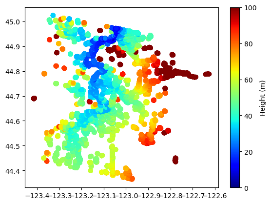
Plot the PIXC data only for good/detected water
This plot is still hard to see, so we will crop around a paticular water-body of interest below
# mask to get good water pixelsmask = np.where(np.logical_and(ds_PIXC.classification >2, ds_PIXC.geolocation_qual <4))plt.scatter(x=ds_PIXC.longitude[mask], y=ds_PIXC.latitude[mask], c=ds_PIXC.height[mask], cmap='jet')plt.clim((0,100))plt.colorbar().set_label('Height (m)')# alternatively wrap the height colorbar at 10m...sometimes this is usefull# (e.g., we want to see fine height structure, but the range of heights is large)#plt.scatter(x=ds_PIXC.longitude[mask], y=ds_PIXC.latitude[mask], c=np.mod(ds_PIXC.height[mask], 10), cmap='hsv')#plt.colorbar().set_label('Height (m), 10 m wrap')
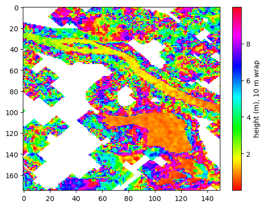
Make function to map a PIXC variable to slant-plane/radar coordiantes
def toslant(pixc, key='height'): az = pixc.azimuth_index.astype(int) rng = pixc.range_index.astype(int) out = np.zeros((pixc.interferogram_size_azimuth +1, pixc.interferogram_size_range +1)) + np.nan var = pixc[key] out[az, rng] = varreturn out
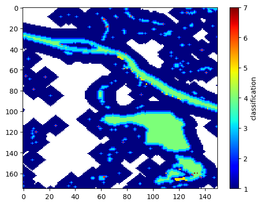
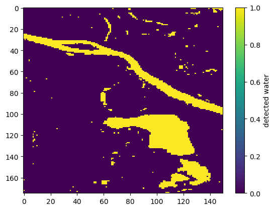
Get the detected water mask from the multi-value class-map and plot it
detected_water = np.zeros(np.shape(klass))detected_water[klass>2] =1detected_water[klass==5] =0# set dark water as not detectedplt.imshow(detected_water, interpolation='none', aspect='auto')plt.colorbar().set_label('detected water')
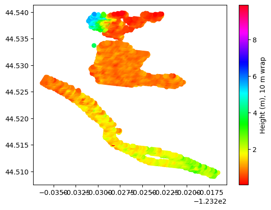
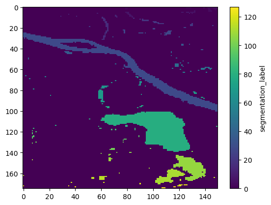
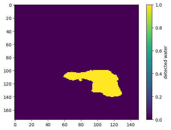
Segment the detected water image to separate out the different water features and focus on just the 1 lake and plot the label image
lake = np.zeros_like(detected_water)lake[lab==79] =1# get the land-near-water pixels toomask = np.zeros_like(detected_water)mask[detected_water==1] =1mask[klass==2] =1iters =range(5)foriterin iters: lake = scipy.ndimage.binary_dilation(lake) lake = lake * masklake[klass<=0] =0plt.imshow(lake, interpolation='none', aspect='auto')plt.colorbar().set_label('detected water')
Mask out relvant variables to get ony lake pixels, where we also have valid SWOT data (in prep to call the RiverObs aggregation functions)
Now we are ready to call the area aggregation function in the RiverObs repo. Note that there is a function that aggregates area-only (SWOTWater.aggregate.area_only()), as well as one that estimates the area uncertainty at the same time (SWOTWater.aggregate.area_with_uncert). Each of them have a ‘method’ parameter that can be set to ‘composite’, ‘water_fraction’, or ‘simple’. For most cases users should apply the ‘composite’ method, which will result in the least bias, while also minimizing the uncertainty.
The ‘composite’ method is what is used in river and lake processors. It directly aggregates the pixel area for interior water (and dark water) pixels, but scales pixel area by the water fraction on the edge pixels (both land near water and water near land).
The ‘water_fraction’ method scales by the water fraction estimate for all pixels
The ‘simple method’ just aggregates the pixel area directly for all detected water pixels
# call the area-only aggregatorarea_comp, num_pixels_comp = SWOTWater.aggregate.area_only( pixel_area_1d, water_frac_1d, klass_1d, good, method='composite')# call the full aggregation method that also computes the area uncertaintyarea_agg, area_unc, area_pcnt_uncert = SWOTWater.aggregate.area_with_uncert( pixel_area_1d, water_frac_1d, water_frac_uncert_1d, darea_dheight_1d, klass_1d, Pfd_1d, Pmd_1d, good, method='composite')
# these other methods are alternatives that have different bias and error characteristics# Users should almost always use the 'composite' method# 'simple' method is just sum of pixel area over the detected water# e.g., detected_area = np.sum(pixel_area_1d[good] * detected_water_1d[good])area_simple, num_pixels_simple = SWOTWater.aggregate.area_only( pixel_area_1d, water_frac_1d, klass_1d, good, method='simple')# 'water_fraction' method is just always scaling by water fraction for detected water and land near waterarea_wf, num_pixels_wf = SWOTWater.aggregate.area_only( pixel_area_1d, water_frac_1d, klass_1d, good, method='water_fraction')
Compare the results from the different methods
# manually do a simple sum of pixel area for comparisondetected_area = np.sum(pixel_area_1d[good] * detected_water_1d[good])# compute area percent diffferentce relative to the 'detected_area'area_perc_diff_comp = (area_comp - detected_area)/np.sqrt(area_comp * detected_area)*100area_perc_diff_simple = (area_simple - detected_area)/np.sqrt(area_simple * detected_area)*100area_perc_diff_wf = (area_wf - detected_area)/np.sqrt(area_wf * detected_area)*100# print out a tableprint("Area estimates:")print("method: \t composite, \t water_fraction, \t simple")print("area: \t{:10.1f}, \t{:10.1f}, \t{:10.1f}".format(area_comp, area_wf, area_simple))print("area_diff:\t{:10.1f}, \t{:10.1f}, \t{:10.1f}".format(area_perc_diff_comp, area_perc_diff_wf, area_perc_diff_simple))