Parallel Computing with Earthdata in the Cloud

Processing a Large Data Set in Chunks Using `coiled.cluster()`, Example Use for an SST Seasonal Cycle Analysis

Authors: Dean Henze, NASA JPL PO.DAAC

Reference herein to any specific commercial product, process, or service by trade name, trademark, manufacturer, or otherwise, does not constitute or imply its endorsement by the United States Government or the Jet Propulsion Laboratory, California Institute of Technology.

Summary

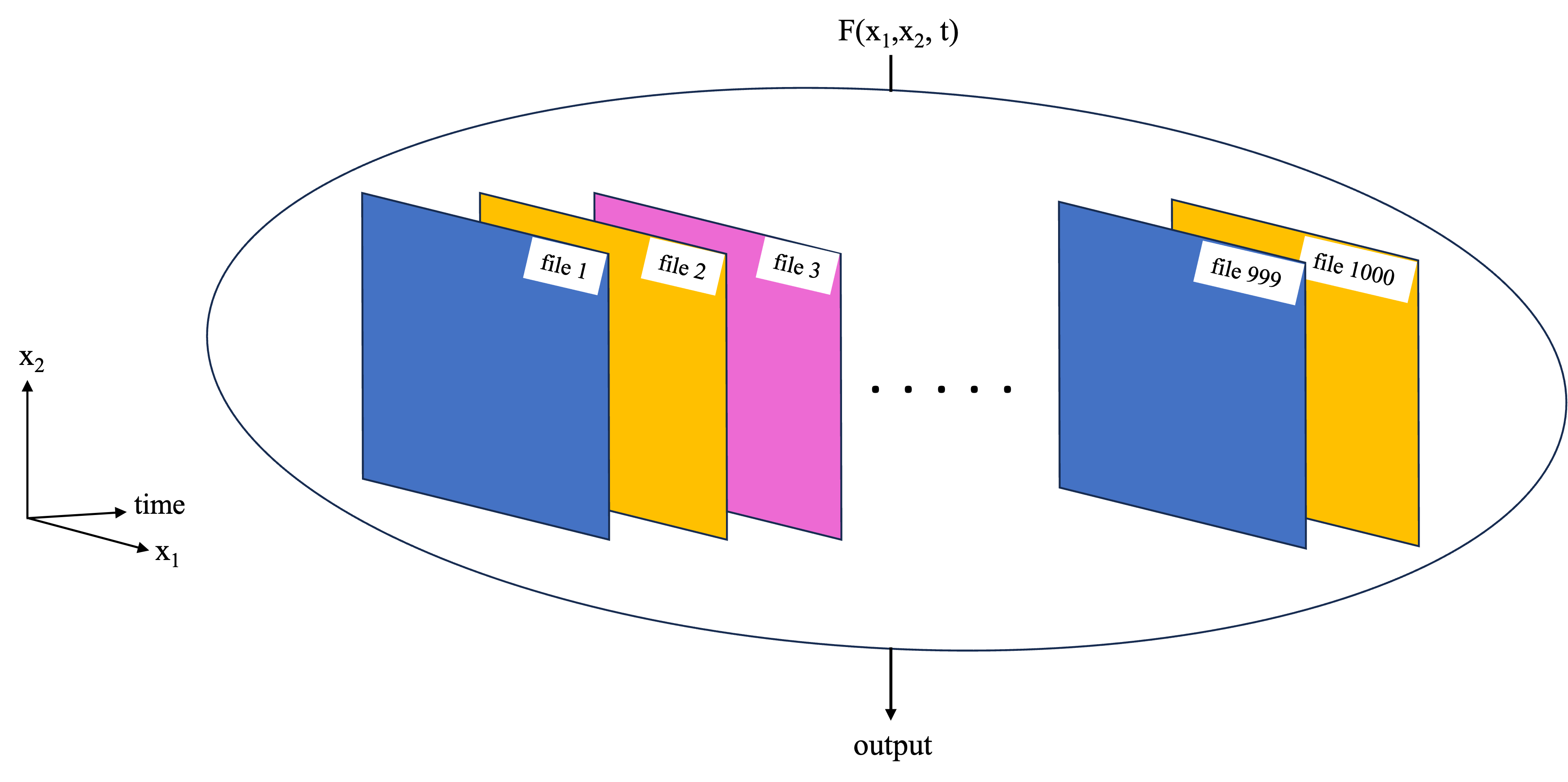
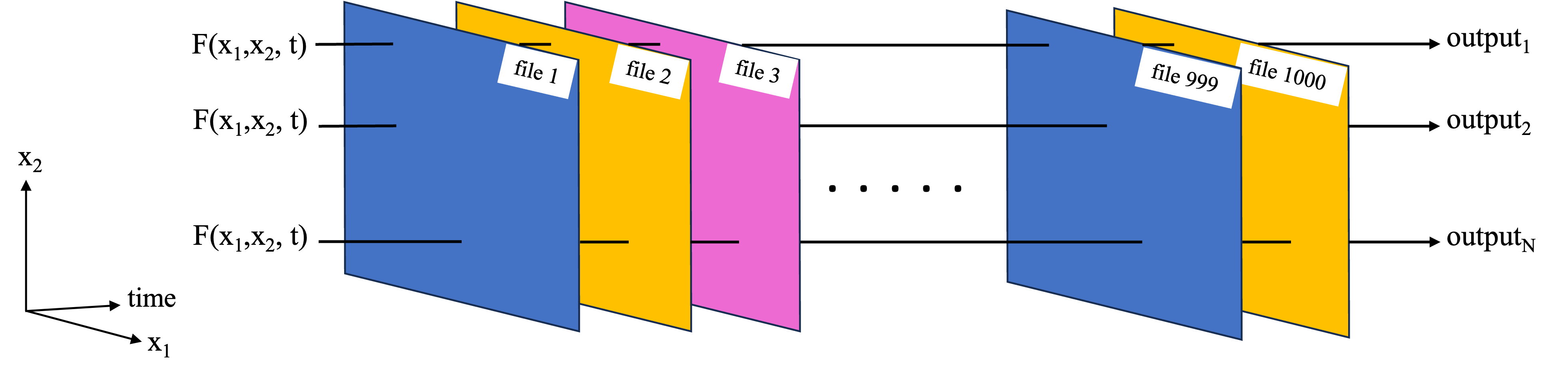
Previous notebooks have covered the use of Dask and parallel computing applied to the type of tasks in the schematic below, where we have a function which needs to work on a large data set as a whole. This could e.g. because the function works on some or all of the data from each of the files, so we can’t just work on each file independently like in the function replication example.

sch1 sch1

In a previous notebook, a toy example was used to demonstrate this basic functionality using a local dask cluster and Xarray built-in functions to work on the data set in chunks. In this notebook, that workflow is expanded to a more complex analysis. Parallel computations are performed via the third party software/package Coiled. In short, Coiled allows us to spin up AWS virtual machines (EC2 instances) and create a distributed cluster out of them, all with a few lines of Python from within a notebook. You will need a Coiled account, but once set up, you can run this notebook entirely from your laptop while the parallel computation portion will be run on the distributed cluster in AWS.

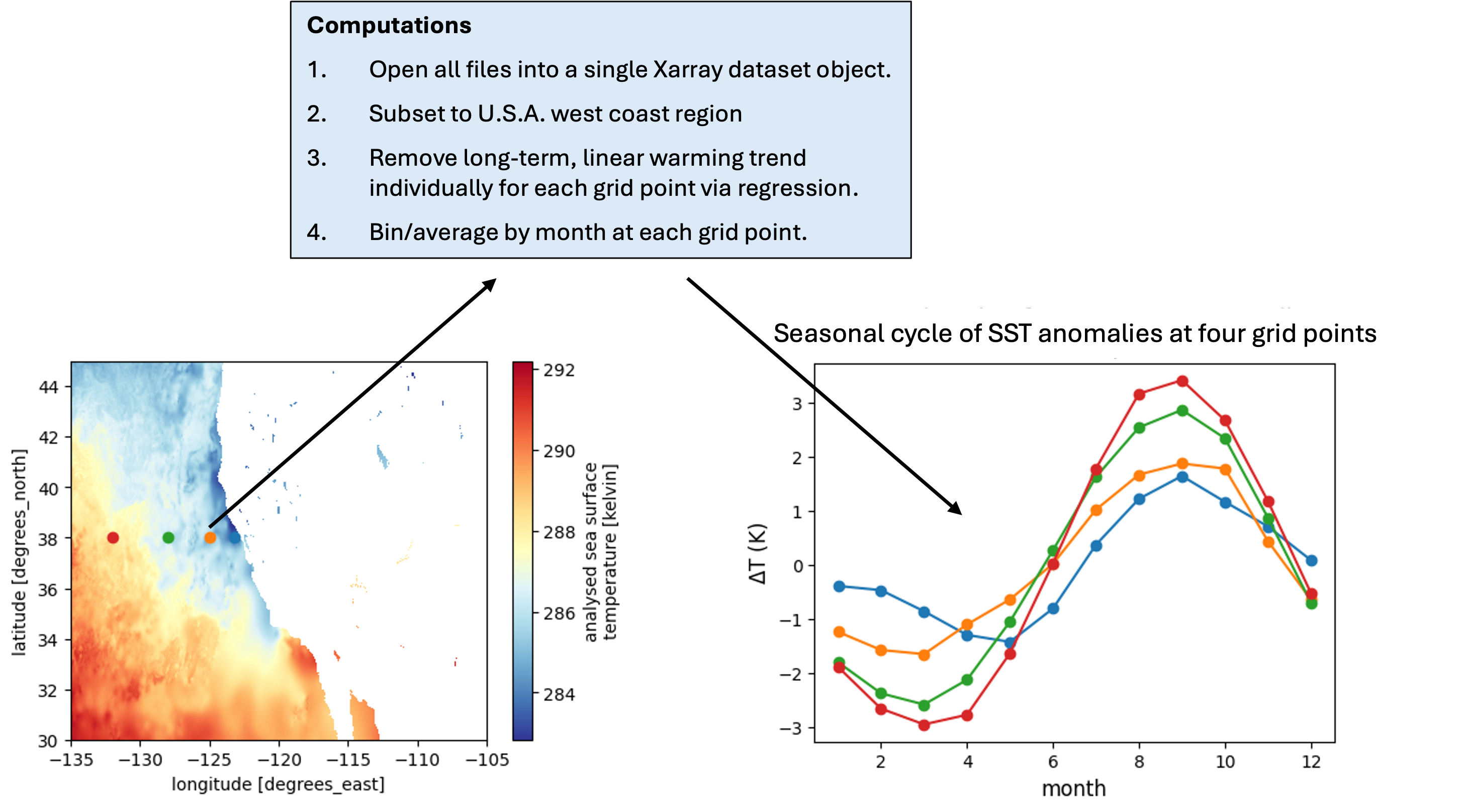
Analysis: Mean Seasonal Cycle of SST Anomalies

The analysis will generate the mean seasonal cycle of sea surface temperature (SST) at each gridpoint in a region of the west coast of the U.S.A. The analysis uses a PO.DAAC hosted gridded global SST data set:

GHRSST Level 4 MUR Global Foundation SST Analysis, V4.1: 0.01° x 0.01° resolution, global map, daily files, https://doi.org/10.5067/GHGMR-4FJ04

The analysis will use files over the first decade of the time record. The following procedure is used to generate seasonal cycles:

sch_sst-ssh-corr

In Section 1 of this notebook, the first decade of MUR files are located on PO.DAAC using the earthaccess package, then a file is inspected and memory requirements for this data set are assessed. In Section 2, a “medium-sized” computation is performed, deriving the mean seasonal cycle for the files thinned out to once per week (570 files, 1.3 TB of uncompressed data) for about $\$$ 0.20. In Section 3, we perform the computation on all the files in the first decade, ~4000 files, ~10 TB of uncompressed data, for about $\$$ 3.

Requirements, prerequisite knowledge, learning outcomes

Requirements to run this notebook

Earthdata login account: An Earthdata Login account is required to access data from the NASA Earthdata system. Please visit https://urs.earthdata.nasa.gov to register and manage your Earthdata Login account.
Coiled account: Create a coiled account (free to sign up), and connect it to an AWS account. For more information on Coiled, setting up an account, and connecting it to an AWS account, see their website https://www.coiled.io.
Compute environment: This notebook can be run either in the cloud (AWS instance running in us-west-2), or on a local compute environment (e.g. laptop, server), but the data loading step currently works substantially faster in the cloud. In both cases, the parallel computations are still sent to VM’s in the cloud.

Prerequisite knowledge

The notebook on Dask basics and all prerequisites therein.

Learning outcomes

This notebook demonstrates how to use Coiled with a distributed cluster to analyze a large data set in chunks, naturally parallelizing Xarray built in functions on the cluster. You will get better insight on how to apply this workflow to your own analysis.

Import packages

We ran this notebook in a Python 3.12.3 environment. The minimal working install we used to run this notebook from a clean environment was:

With pip:

pip install xarray==2024.1.0 numpy==1.26.3 h5netcdf==1.3.0 "dask[complete]"==2024.5.2 earthaccess==0.9.0 matplotlib==3.8.0 coiled==1.28.0 jupyterlab

or with conda:

conda install -c conda-forge xarray==2024.1.0 numpy==1.26.3 h5netcdf==1.3.0 dask==2024.5.2 earthaccess==0.9.0 matplotlib==3.8.0 coiled==1.28.0 jupyterlab

# NASA data access packages:
import earthaccess

# Analysis packages:
import xarray as xr
import numpy as np                 

# Visualization packages:
import matplotlib.pyplot as plt
%matplotlib inline

# Cloud computing / dask packages:
import coiled

xr.set_options( # display options for xarray objects
    display_expand_attrs=False,
    display_expand_coords=True,
    display_expand_data=True,
)

<xarray.core.options.set_options at 0x7f89550bbfb0>

1. Locate MUR SST file access endpoints for first decade of record, inspect a file

We use earthaccess to find metadata and endpoints for the files.

earthaccess.login() # Login with your credentials

Enter your Earthdata Login username:  deanh808
Enter your Earthdata password:  ········

<earthaccess.auth.Auth at 0x7f897ede49b0>

datainfo = earthaccess.search_data(
    short_name="MUR-JPL-L4-GLOB-v4.1",
    cloud_hosted=True,
    temporal=("2002-01-01", "2013-05-01"),
    )

Granules found: 3988

Open and inspect a file

Open a file and plot the SST data in the region for our analysis.

fileobj_test = earthaccess.open([datainfo[0]])[0] # Generate file-like objects compatible with Xarray
sst_test = xr.open_dataset(fileobj_test)['analysed_sst']
sst_test

Opening 1 granules, approx size: 0.32 GB
using endpoint: https://archive.podaac.earthdata.nasa.gov/s3credentials

# Region to perform analysis over:
lat_region = (30, 45)
lon_region = (-135, -105)

## Plot SST in analysis region:
fig = plt.figure()
sst_test.sel(lat=slice(*lat_region), lon=slice(*lon_region)).plot(cmap='RdYlBu_r')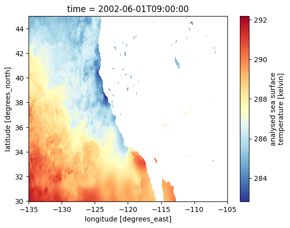

Memory considerations

Demonstrating that these are fairly large files, especially uncompressed, at the time this notebook was written:

print("Disk size of one file =", datainfo[0]['size'], "MB.")

Disk size of one file = 332.3598403930664 MB.

print("Size in-memory of the SST variable once uncompressed =", sst_test.nbytes/10**9, "GB.")

Size in-memory of the SST variable once uncompressed = 2.591856 GB.

At ~2.5 GB uncompressed, and ~4000 MUR files at the time this notebook was written, we are dealing with a ~10 TB data set.

2. Seasonal cycle at weekly temporal resolution

For this “medium-sized” computation, the decade time record is thinned out to one file per week. This will be ~200 GB on disk, and ~1.3 TB uncompressed in memory. Using the parallel computing methods below, we were able to accomplish this in about 4 minutes for \$0.20 (1 minute for opening the data set and 3 minutes for computations). For the size of this computation, we obtained good results with 25 compute-optimized c7g.large VMs. For the larger computation in Section 3, we switch to memory-optimized VMs.

# Thin to weekly temporal resolution:
datainfo_thinned = [datainfo[i] for i in range(len(datainfo)) if i%7==0]

# Confirm we have about a decade of files at weekly resolution:
print("First and last file times \n--------------------------")
print(datainfo_thinned[0]['umm']['TemporalExtent']['RangeDateTime']['BeginningDateTime'])
print(datainfo_thinned[-1]['umm']['TemporalExtent']['RangeDateTime']['BeginningDateTime'])
print("\nFirst and second file times \n--------------------------")
print(datainfo_thinned[0]['umm']['TemporalExtent']['RangeDateTime']['BeginningDateTime'])
print(datainfo_thinned[1]['umm']['TemporalExtent']['RangeDateTime']['BeginningDateTime'])

First and last file times 
--------------------------
2002-05-31T21:00:00.000Z
2013-04-26T21:00:00.000Z

First and second file times 
--------------------------
2002-05-31T21:00:00.000Z
2002-06-07T21:00:00.000Z

Since Xarray built-in functions are used to both open and process the data, the workflow is to start up a cluster, open the files into a single dataset with chunking, and then Xarray function calls will naturally be run in parallel on the cluster.

fileobjs = earthaccess.open(datainfo_thinned) # Generate file objects from the endpoints which are compatible with Xarray

Opening 570 granules, approx size: 190.08 GB
using endpoint: https://archive.podaac.earthdata.nasa.gov/s3credentials

CPU times: user 1.03 s, sys: 70.6 ms, total: 1.1 s
Wall time: 1.55 s

cluster = coiled.Cluster(
    n_workers=25, 
    region="us-west-2", 
    worker_vm_types="c7g.large", # or can try "m7a.medium"
    scheduler_vm_types="c7g.large" # or can try "m7a.medium"
    ) 
client = cluster.get_client()

╭────────────────────────── Not Synced with Cluster ───────────────────────────╮
│             ╷                                                    ╷           │
│   Package   │ Error                                              │ Risk      │
│ ╶───────────┼────────────────────────────────────────────────────┼─────────╴ │
│   libcxxabi │ libcxxabi~=17.0.6 has no install candidate for     │ Warning   │
│             │ Python 3.12 linux-aarch64 on conda-forge           │           │
│             ╵                                                    ╵           │
╰──────────────────────────────────────────────────────────────────────────────╯

%%time

## Load files and rechunk SST data:
murdata = xr.open_mfdataset(fileobjs, parallel=True, chunks={'lat': 6000, 'lon': 6000, 'time': 1})
sst = murdata["analysed_sst"]
    # Rechunk to get bigger slices along time dimension, since many of the computations
    # operate along that axis:
sst = sst.chunk(chunks={'lat': 500, 'lon': 500, 'time': 200})
sst

CPU times: user 9.23 s, sys: 564 ms, total: 9.79 s
Wall time: 51.2 s

<xarray.DataArray 'analysed_sst' (time: 570, lat: 17999, lon: 36000)>
dask.array<rechunk-merge, shape=(570, 17999, 36000), dtype=float32, chunksize=(200, 500, 500), chunktype=numpy.ndarray>
Coordinates:
  * time     (time) datetime64[ns] 2002-06-01T09:00:00 ... 2013-04-27T09:00:00
  * lat      (lat) float32 -89.99 -89.98 -89.97 -89.96 ... 89.97 89.98 89.99
  * lon      (lon) float32 -180.0 -180.0 -180.0 -180.0 ... 180.0 180.0 180.0
Attributes: (7)

Computations

We chose not to suppress the large chunk and task graph warnings for the next two blocks:

## ----------------
## Set up analysis
## ----------------
## (Since these are dask arrays, functions calls don't do the computations yet, just set them up)

## Subset to region off U.S.A. west coast:
sst_regional = sst.sel(lat=slice(*lat_region), lon=slice(*lon_region))

## Remove linear warming trend:
p = sst_regional.polyfit(dim='time', deg=1) # Deg 1 poly fit coefficients at each grid point.
fit = xr.polyval(sst_regional['time'], p.polyfit_coefficients) # Linear fit time series at each point.
sst_detrend = (sst_regional - fit) # xarray is smart enough to subtract along the time dim.

## Mean seasonal cycle:
seasonal_cycle = sst_detrend.groupby("time.month").mean("time")

/opt/coiled/env/lib/python3.12/site-packages/xarray/core/dataset.py:5196: PerformanceWarning: Reshaping is producing a large chunk. To accept the large
chunk and silence this warning, set the option
    >>> with dask.config.set(**{'array.slicing.split_large_chunks': False}):
    ...     array.reshape(shape)

To avoid creating the large chunks, set the option
    >>> with dask.config.set(**{'array.slicing.split_large_chunks': True}):
    ...     array.reshape(shape)Explicitly passing ``limit`` to ``reshape`` will also silence this warning
    >>> array.reshape(shape, limit='128 MiB')
  stacked_var = exp_var.stack(**{new_dim: dims})

%%time
## ----------------
## Compute it all!!
## ----------------
seasonal_cycle = seasonal_cycle.compute()
cluster.scale(1)

/opt/coiled/env/lib/python3.12/site-packages/distributed/client.py:3161: UserWarning: Sending large graph of size 32.08 MiB.
This may cause some slowdown.
Consider scattering data ahead of time and using futures.
  warnings.warn(

CPU times: user 2.25 s, sys: 559 ms, total: 2.81 s
Wall time: 3min 54s

client.shutdown()
cluster.shutdown()

Plot results

# Points to plot seasonal cycle at:
lat_points = (38, 38, 38, 38)
lon_points = (-123.25, -125, -128, -132)

fig2, axes2 = plt.subplots(1, 2, figsize=(12, 4))

## Replot the map and points from the test file:
sst_test.sel(lat=slice(*lat_region), lon=slice(*lon_region)).plot(ax=axes2[0], cmap='RdYlBu_r')
for lat, lon in zip(lat_points, lon_points):
    axes2[0].scatter(lon, lat)

## Seasonal cycles on another plot
for lat, lon in zip(lat_points, lon_points):
    scycle_point = seasonal_cycle.sel(lat=lat, lon=lon)
    axes2[1].plot(scycle_point['month'], scycle_point.values, 'o-')

axes2[1].set_title("Seasonal cycle of temperature anomalies \n at four test points", fontsize=14)
axes2[1].set_xlabel("month", fontsize=12)
axes2[1].set_ylabel(r"$\Delta$T (K)", fontsize=12)

Text(0, 0.5, '$\\Delta$T (K)')

3. Seasonal cycle for full record (daily resolution)

Section 1 needs to be run prior to this one, but Section 2 can be skipped.

In this section, all files in the decade are processed. This will be ~4000 files, ~1.3 TB on disk, and ~10 TB for the SST varaible once uncompressed in memory. Using the parallel computing methods below (with 40 r7g.xlarge VMs), we were able to accomplish this in about 20 minutes for \$3 (5 minutes for opening the data set and 15 minutes for computations).

For this computation, memory-optimized VMs were chosen (they have high memory per CPU), following the example Coiled post here. In short, it is more efficient to create larger chunks and have VMs which can handle the larger chunks.

fileobjs = earthaccess.open(datainfo) # Generate file-like objects compatible with Xarray

Opening 3988 granules, approx size: 1330.13 GB
using endpoint: https://archive.podaac.earthdata.nasa.gov/s3credentials

cluster = coiled.Cluster(
    n_workers=40, 
    region="us-west-2", 
    worker_vm_types="r7g.xlarge",
    scheduler_vm_types="r7g.xlarge"
    ) 
client = cluster.get_client()

╭────────────────────────── Not Synced with Cluster ───────────────────────────╮
│             ╷                                                    ╷           │
│   Package   │ Error                                              │ Risk      │
│ ╶───────────┼────────────────────────────────────────────────────┼─────────╴ │
│   libcxxabi │ libcxxabi~=17.0.6 has no install candidate for     │ Warning   │
│             │ Python 3.12 linux-aarch64 on conda-forge           │           │
│             ╵                                                    ╵           │
╰──────────────────────────────────────────────────────────────────────────────╯

%%time

## Load files and rechunk SST data:
murdata = xr.open_mfdataset(fileobjs, parallel=True, chunks={'lat': 6000, 'lon': 6000, 'time': 1})
sst = murdata["analysed_sst"]
    # Rechunk to get bigger slices along time dimension, since many of our computations are
    # operating along that axis:
sst = sst.chunk(chunks={'lat': 500, 'lon': 500, 'time': 400})
sst

/opt/coiled/env/lib/python3.12/site-packages/distributed/client.py:3161: UserWarning: Sending large graph of size 18.07 MiB.
This may cause some slowdown.
Consider scattering data ahead of time and using futures.
  warnings.warn(

CPU times: user 55.3 s, sys: 3.72 s, total: 59 s
Wall time: 5min 1s

<xarray.DataArray 'analysed_sst' (time: 3988, lat: 17999, lon: 36000)>
dask.array<rechunk-merge, shape=(3988, 17999, 36000), dtype=float32, chunksize=(400, 500, 500), chunktype=numpy.ndarray>
Coordinates:
  * time     (time) datetime64[ns] 2002-06-01T09:00:00 ... 2013-05-01T09:00:00
  * lat      (lat) float32 -89.99 -89.98 -89.97 -89.96 ... 89.97 89.98 89.99
  * lon      (lon) float32 -180.0 -180.0 -180.0 -180.0 ... 180.0 180.0 180.0
Attributes: (7)

Computations

We chose not to suppress the large chunk and task graph warnings for the next two blocks:

## ----------------
## Set up analysis
## ----------------
## (Since these are dask arrays, functions calls don't do the computations yet, just set them up)

## Subset to region off U.S.A. west coast:
sst_regional = sst.sel(lat=slice(*lat_region), lon=slice(*lon_region))

## Remove linear warming trend:
p = sst_regional.polyfit(dim='time', deg=1) # Deg 1 poly fit coefficients at each grid point.
fit = xr.polyval(sst_regional['time'], p.polyfit_coefficients) # Linear fit time series at each point.
sst_detrend = (sst_regional - fit) # xarray is smart enough to subtract along the time dim.

## Mean seasonal cycle:
seasonal_cycle = sst_detrend.groupby("time.month").mean("time")

/opt/coiled/env/lib/python3.12/site-packages/xarray/core/dataset.py:5196: PerformanceWarning: Reshaping is producing a large chunk. To accept the large
chunk and silence this warning, set the option
    >>> with dask.config.set(**{'array.slicing.split_large_chunks': False}):
    ...     array.reshape(shape)

To avoid creating the large chunks, set the option
    >>> with dask.config.set(**{'array.slicing.split_large_chunks': True}):
    ...     array.reshape(shape)Explicitly passing ``limit`` to ``reshape`` will also silence this warning
    >>> array.reshape(shape, limit='128 MiB')
  stacked_var = exp_var.stack(**{new_dim: dims})

%%time
## ----------------
## Compute it all!!
## ----------------
seasonal_cycle = seasonal_cycle.compute()
cluster.scale(1)

/opt/coiled/env/lib/python3.12/site-packages/distributed/client.py:3161: UserWarning: Sending large graph of size 225.00 MiB.
This may cause some slowdown.
Consider scattering data ahead of time and using futures.
  warnings.warn(

CPU times: user 11.1 s, sys: 1.05 s, total: 12.1 s
Wall time: 14min 16s

client.shutdown()
cluster.shutdown()

Plot results

# Points to plot seasonal cycle at:
lat_points = (38, 38, 38, 38)
lon_points = (-123.25, -125, -128, -132)

fig2, axes2 = plt.subplots(1, 2, figsize=(12, 4))

## Replot the map and points from the test file:
sst_test.sel(lat=slice(*lat_region), lon=slice(*lon_region)).plot(ax=axes2[0], cmap='RdYlBu_r')
for lat, lon in zip(lat_points, lon_points):
    axes2[0].scatter(lon, lat)

## Seasonal cycles on another plot
for lat, lon in zip(lat_points, lon_points):
    scycle_point = seasonal_cycle.sel(lat=lat, lon=lon)
    axes2[1].plot(scycle_point['month'], scycle_point.values, 'o-')

axes2[1].set_title("Seasonal cycle of temperature anomalies \n at four test points", fontsize=14)
axes2[1].set_xlabel("month", fontsize=12)
axes2[1].set_ylabel(r"$\Delta$T (K)", fontsize=12)

Text(0, 0.5, '$\\Delta$T (K)')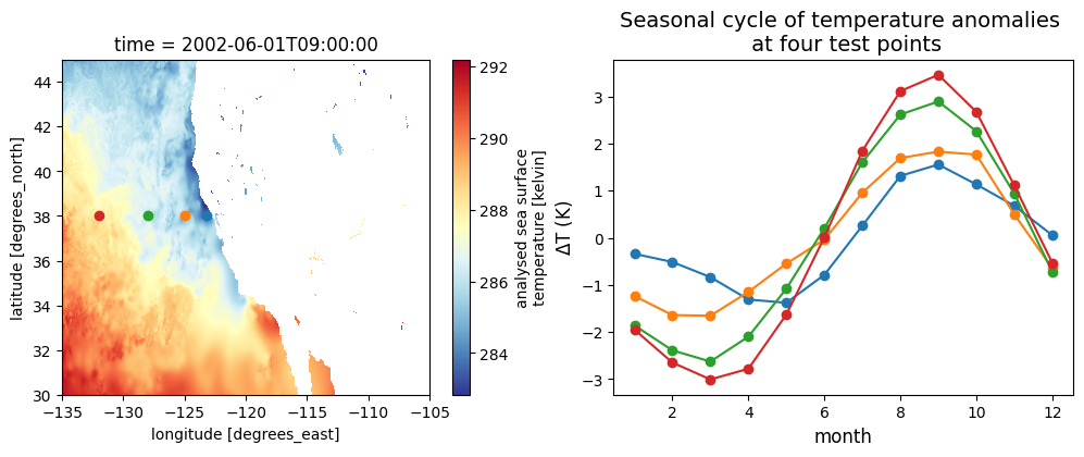

4. Additional Notes

To compute the mean seasonal cycle, Xarray’s built in groupby() function is used to group the data by month of the year. As per this Xarray docs page, one can try using the flox package to speed up this groupby operation.

Processing a Large Data Set in Chunks Using coiled.cluster(), Example Use for an SST Seasonal Cycle Analysis

Authors: Dean Henze, NASA JPL PO.DAAC

Summary

Analysis: Mean Seasonal Cycle of SST Anomalies

Requirements, prerequisite knowledge, learning outcomes

Requirements to run this notebook

Prerequisite knowledge

Learning outcomes

Import packages

1. Locate MUR SST file access endpoints for first decade of record, inspect a file

Open and inspect a file

Memory considerations

2. Seasonal cycle at weekly temporal resolution

Plot results

3. Seasonal cycle for full record (daily resolution)

Plot results

4. Additional Notes

Processing a Large Data Set in Chunks Using `coiled.cluster()`, Example Use for an SST Seasonal Cycle Analysis