From the PO.DAAC Cookbook, to access the GitHub version of the notebook, follow this link.

Amazon Estuary Exploration:

In AWS Cloud Version

This tutorial is one of two jupyter notebook versions of the same use case exploring multiple satellite data products over the Amazon Estuary. In this version, we use data products directly in the Amazon Web Services (AWS) Cloud.

Learning Objectives

• Compare cloud access methods (in tandem with notebook “Amazon Estuary Exploration: Cloud Direct Download Version”)
• Search for data products using earthaccess Python library
• Access datasets using direct s3 access in cloud, xarray and visualize using hvplot or plot tools

This tutorial explores the relationships between river height, land water equivalent thickness, sea surface salinity, and sea surface temperature in the Amazon River estuary and coastal region from multiple datasets listed below. The contents are useful for the ocean, coastal, and terrestrial hydrosphere communities, showcasing how to use cloud datasets and services. The notebook is designed to be executed in Amazon Web Services (AWS) (in us-west-2 region where the cloud data is located).

Cloud Datasets

The tutorial itself will use four different datasets:

1. TELLUS_GRAC-GRFO_MASCON_CRI_GRID_RL06.1_V3

DOI: https://doi.org/10.5067/TEMSC-3JC63

The Gravity Recovery And Climate Experiment Follow-On (GRACE-FO) satellite land water equivalent (LWE) thicknesses will be used to observe seasonal changes in water storage around the river. When discharge is high, the change in water storage will increase, thus highlighting a wet season. 

2. PRESWOT_HYDRO_GRRATS_L2_DAILY_VIRTUAL_STATION_HEIGHTS_V2

DOI: https://doi.org/10.5067/PSGRA-DA2V2

The NASA Pre-SWOT Making Earth System Data Records for Use in Research Environments (MEaSUREs) Program virtual gauges will be used as a proxy for Surface Water and Ocean Topography (SWOT) discharge until SWOT products are available. MEaSUREs contains river height products, not discharge, but river height is directly related to discharge and thus will act as a good substitute.

3. OISSS_L4_multimission_7day_v1

DOI: https://doi.org/10.5067/SMP10-4U7CS

Optimally Interpolated Sea surface salinity (OISSS) is a level 4 product that combines the records from Aquarius (Sept 2011-June 2015), the Soil Moisture Active Passive (SMAP) satellite (April 2015-present), and ESAs Soil Moisture Ocean Salinity (SMOS) data to fill in data gaps.

4. MODIS_AQUA_L3_SST_MID-IR_MONTHLY_9KM_NIGHTTIME_V2019.0

DOI: https://doi.org/10.5067/MODAM-MO9N9

Sea surface temperature is obtained from the Moderate Resolution Imaging Spectrometer (MODIS) instrument on board the Aqua satellite. 

More details on available collections are on the PO.DAAC Cloud Earthdata Search Portal. For more information on the PO.DAAC transition to the cloud, please visit: https://podaac.jpl.nasa.gov/cloud-datasets/about

Needed Packages

import os
import glob
import s3fs
import requests
import numpy as np
import pandas as pd
import xarray as xr
import hvplot.xarray
import matplotlib.pyplot as plt
import cartopy.crs as ccrs
import cartopy
import dask
from datetime import datetime
from os.path import isfile, basename, abspath
import earthaccess
from earthaccess import Auth, DataCollections, DataGranules, Store

Earthdata Login

An Earthdata Login account is required to access data, as well as discover restricted data, from the NASA Earthdata system. Thus, to access NASA data, you need Earthdata Login. Please visit https://urs.earthdata.nasa.gov to register and manage your Earthdata Login account. This account is free to create and only takes a moment to set up. We use earthaccess to authenticate your login credentials below.

auth = earthaccess.login(strategy="interactive", persist=True)

Liquid Water Equivalent (LWE) Thickness (GRACE & GRACE-FO)

Search for GRACE LWE Thickness data

Suppose we are interested in LWE data from the dataset (DOI:10.5067/TEMSC-3JC63) described on this PO.DAAC dataset landing page: https://podaac.jpl.nasa.gov/dataset/TELLUS_GRAC-GRFO_MASCON_CRI_GRID_RL06.1_V3 From the landing page, we see the dataset Short Name under the Information tab. This is what we will be using to search for the collection with earthaccess.

You can also access the short name of the dataset through Earthdata search at: https://search.earthdata.nasa.gov.

#search for the granules using the short name
grace_results = earthaccess.search_data(short_name="TELLUS_GRAC-GRFO_MASCON_CRI_GRID_RL06.1_V3")

Granules found: 1

Open the .nc file in the s3 bucket and load it into an xarray dataset

ds_GRACE = xr.open_mfdataset(earthaccess.open([grace_results[0]]), engine='h5netcdf')
ds_GRACE

 Opening 1 granules, approx size: 0.0 GB

<xarray.Dataset>
Dimensions:        (lon: 720, lat: 360, time: 219, bounds: 2)
Coordinates:
  * lon            (lon) float64 0.25 0.75 1.25 1.75 ... 358.2 358.8 359.2 359.8
  * lat            (lat) float64 -89.75 -89.25 -88.75 ... 88.75 89.25 89.75
  * time           (time) datetime64[ns] 2002-04-17T12:00:00 ... 2023-03-16T1...
Dimensions without coordinates: bounds
Data variables:
    lwe_thickness  (time, lat, lon) float64 dask.array<chunksize=(219, 360, 720), meta=np.ndarray>
    uncertainty    (time, lat, lon) float64 dask.array<chunksize=(219, 360, 720), meta=np.ndarray>
    lat_bounds     (lat, bounds) float64 dask.array<chunksize=(360, 2), meta=np.ndarray>
    lon_bounds     (lon, bounds) float64 dask.array<chunksize=(720, 2), meta=np.ndarray>
    time_bounds    (time, bounds) datetime64[ns] dask.array<chunksize=(219, 2), meta=np.ndarray>
    land_mask      (lat, lon) float64 dask.array<chunksize=(360, 720), meta=np.ndarray>
    scale_factor   (lat, lon) float64 dask.array<chunksize=(360, 720), meta=np.ndarray>
    mascon_ID      (lat, lon) float64 dask.array<chunksize=(360, 720), meta=np.ndarray>
Attributes: (12/53)
    Conventions:                   CF-1.6, ACDD-1.3, ISO 8601
    Metadata_Conventions:          Unidata Dataset Discovery v1.0
    standard_name_vocabulary:      NetCDF Climate and Forecast (CF) Metadata ...
    title:                         JPL GRACE and GRACE-FO MASCON RL06.1Mv03 CRI
    summary:                       Monthly gravity solutions from GRACE and G...
    keywords:                      Solid Earth, Geodetics/Gravity, Gravity, l...
    ...                            ...
    C_30_substitution:             TN-14; Loomis et al., 2019, Geophys. Res. ...
    user_note_1:                   The accelerometer on the GRACE-B spacecraf...
    user_note_2:                   The accelerometer on the GRACE-D spacecraf...
    journal_reference:             Watkins, M. M., D. N. Wiese, D.-N. Yuan, C...
    CRI_filter_journal_reference:  Wiese, D. N., F. W. Landerer, and M. M. Wa...
    date_created:                  2023-05-22T06:05:03Z

xarray.Dataset

• Dimensions:
  • lon: 720
  • lat: 360
  • time: 219
  • bounds: 2
• Coordinates: (3)
  • lon
    (lon)
    float64
    0.25 0.75 1.25 ... 359.2 359.8

    units :

    degrees_east

    long_name :

    longitude

    standard_name :

    longitude

    axis :

    X

    valid_min :

    0.25

    valid_max :

    359.75

    bounds :

    lon_bounds

    array([2.5000e-01, 7.5000e-01, 1.2500e+00, ..., 3.5875e+02, 3.5925e+02,
           3.5975e+02])

  • lat
    (lat)
    float64
    -89.75 -89.25 ... 89.25 89.75

    units :

    degrees_north

    long_name :

    latitude

    standard_name :

    latitude

    axis :

    Y

    valid_min :

    -89.75

    valid_max :

    89.75

    bounds :

    lat_bounds

    array([-89.75, -89.25, -88.75, ...,  88.75,  89.25,  89.75])

  • time
    (time)
    datetime64[ns]
    2002-04-17T12:00:00 ... 2023-03-...

    long_name :

    time

    standard_name :

    time

    axis :

    T

    bounds :

    time_bounds

    array(['2002-04-17T12:00:00.000000000', '2002-05-10T12:00:00.000000000',
           '2002-08-16T12:00:00.000000000', ..., '2023-01-16T12:00:00.000000000',
           '2023-02-15T00:00:00.000000000', '2023-03-16T12:00:00.000000000'],
          dtype='datetime64[ns]')

• Data variables: (8)
  • lwe_thickness
    (time, lat, lon)
    float64
    dask.array<chunksize=(219, 360, 720), meta=np.ndarray>

    units :

    cm

    long_name :

    Liquid_Water_Equivalent_Thickness

    standard_name :

    Liquid_Water_Equivalent_Thickness

    grid_mapping :

    WGS84

    valid_min :

    -1986.9763606523888

    valid_max :

    965.4782725418918

    comment :

    Coastline Resolution Improvement (CRI) filter is applied

    Array Chunk Bytes 433.08 MiB 433.08 MiB Shape (219, 360, 720) (219, 360, 720) Dask graph 1 chunks in 2 graph layers Data type float64 numpy.ndarray

  • uncertainty
    (time, lat, lon)
    float64
    dask.array<chunksize=(219, 360, 720), meta=np.ndarray>

    units :

    cm

    long_name :

    uncertainty

    standard_name :

    uncertainty

    grid_mapping :

    WGS84

    valid_min :

    0.15854006805783352

    valid_max :

    53.34469598560085

    comment :

    1-sigma uncertainty: not for each 0.5 degree grid cell, but for each 3-degree mascon estimate

    Array Chunk Bytes 433.08 MiB 433.08 MiB Shape (219, 360, 720) (219, 360, 720) Dask graph 1 chunks in 2 graph layers Data type float64 numpy.ndarray

  • lat_bounds
    (lat, bounds)
    float64
    dask.array<chunksize=(360, 2), meta=np.ndarray>

    long_name :

    latitude boundaries

    units :

    degrees_north

    comment :

    latitude values at the north and south bounds of each pixel

    Array Chunk Bytes 5.62 kiB 5.62 kiB Shape (360, 2) (360, 2) Dask graph 1 chunks in 2 graph layers Data type float64 numpy.ndarray

  • lon_bounds
    (lon, bounds)
    float64
    dask.array<chunksize=(720, 2), meta=np.ndarray>

    long_name :

    longitude boundaries

    units :

    degrees_east

    comment :

    longitude values at the west and east bounds of each pixel

    Array Chunk Bytes 11.25 kiB 11.25 kiB Shape (720, 2) (720, 2) Dask graph 1 chunks in 2 graph layers Data type float64 numpy.ndarray

  • time_bounds
    (time, bounds)
    datetime64[ns]
    dask.array<chunksize=(219, 2), meta=np.ndarray>

    long_name :

    time boundaries

    comment :

    time bounds for each time value, i.e. the first day and last day included in the monthly solution

    Array Chunk Bytes 3.42 kiB 3.42 kiB Shape (219, 2) (219, 2) Dask graph 1 chunks in 2 graph layers Data type datetime64[ns] numpy.ndarray

  • land_mask
    (lat, lon)
    float64
    dask.array<chunksize=(360, 720), meta=np.ndarray>

    units :

    binary

    long_name :

    Land_Mask

    standard_name :

    Land_Mask

    description :

    Land Mask that was used with the CRI filter

    Array Chunk Bytes 1.98 MiB 1.98 MiB Shape (360, 720) (360, 720) Dask graph 1 chunks in 2 graph layers Data type float64 numpy.ndarray

  • scale_factor
    (lat, lon)
    float64
    dask.array<chunksize=(360, 720), meta=np.ndarray>

    units :

    dimensionless

    long_name :

    Scale_Factor_CRI

    standard_name :

    Scale_Factor_CRI

    valid_min :

    -99999.0

    valid_max :

    24.133988467789724

    description :

    Gridded scale factors to be used with mascon solution that has the CRI filter applied; based on CLM data from 2002-2009

    Array Chunk Bytes 1.98 MiB 1.98 MiB Shape (360, 720) (360, 720) Dask graph 1 chunks in 2 graph layers Data type float64 numpy.ndarray

  • mascon_ID
    (lat, lon)
    float64
    dask.array<chunksize=(360, 720), meta=np.ndarray>

    units :

    dimensionless

    long_name :

    Mascon_Identifier

    standard_name :

    Mascon_ID

    valid_min :

    1

    valid_max :

    4551

    description :

    Mascon identifier mapped to the grid

    Array Chunk Bytes 1.98 MiB 1.98 MiB Shape (360, 720) (360, 720) Dask graph 1 chunks in 2 graph layers Data type float64 numpy.ndarray

• Indexes: (3)
  • lon
    PandasIndex

    PandasIndex(Index([  0.25,   0.75,   1.25,   1.75,   2.25,   2.75,   3.25,   3.75,   4.25,
             4.75,
           ...
           355.25, 355.75, 356.25, 356.75, 357.25, 357.75, 358.25, 358.75, 359.25,
           359.75],
          dtype='float64', name='lon', length=720))

  • lat
    PandasIndex

    PandasIndex(Index([-89.75, -89.25, -88.75, -88.25, -87.75, -87.25, -86.75, -86.25, -85.75,
           -85.25,
           ...
            85.25,  85.75,  86.25,  86.75,  87.25,  87.75,  88.25,  88.75,  89.25,
            89.75],
          dtype='float64', name='lat', length=360))

  • time
    PandasIndex

    PandasIndex(DatetimeIndex(['2002-04-17 12:00:00', '2002-05-10 12:00:00',
                   '2002-08-16 12:00:00', '2002-09-16 00:00:00',
                   '2002-10-16 12:00:00', '2002-11-16 00:00:00',
                   '2002-12-16 12:00:00', '2003-01-16 12:00:00',
                   '2003-02-15 00:00:00', '2003-03-16 12:00:00',
                   ...
                   '2022-06-16 00:00:00', '2022-07-16 12:00:00',
                   '2022-08-16 12:00:00', '2022-09-16 00:00:00',
                   '2022-10-16 12:00:00', '2022-11-16 00:00:00',
                   '2022-12-16 12:00:00', '2023-01-16 12:00:00',
                   '2023-02-15 00:00:00', '2023-03-16 12:00:00'],
                  dtype='datetime64[ns]', name='time', length=219, freq=None))

• Attributes: (53)

  Conventions :

  CF-1.6, ACDD-1.3, ISO 8601

  Metadata_Conventions :

  Unidata Dataset Discovery v1.0

  standard_name_vocabulary :

  NetCDF Climate and Forecast (CF) Metadata Convention-1.6

  title :

  JPL GRACE and GRACE-FO MASCON RL06.1Mv03 CRI

  summary :

  Monthly gravity solutions from GRACE and GRACE-FO as determined from the JPL RL06.1Mv03 mascon solution - with CRI filter applied

  keywords :

  Solid Earth, Geodetics/Gravity, Gravity, liquid_water_equivalent_thickness

  keywords_vocabulary :

  NASA Global Change Master Directory (GCMD) Science Keywords

  platform :

  GRACE and GRACE-FO

  institution :

  NASA/JPL

  creator_name :

  David Wiese

  creator_email :

  grace@podaac.jpl.nasa.gov

  creator_url :

  https://grace.jpl.nasa.gov

  creator_type :

  group

  creator_institution :

  NASA/JPL

  publisher_name :

  Physical Oceanography Distributed Active Archive Center

  publisher_email :

  podaac@jpl.nasa.gov

  publisher_url :

  https://podaac.jpl.nasa.gov

  publisher_type :

  group

  publisher_institution :

  NASA/JPL

  project :

  NASA Gravity Recovery and Climate Experiment (GRACE) and NASA Gravity Recovery and Climate Experiment Follow-On (GRACE-FO)

  program :

  NASA Earth Science System Pathfinder and NASA Earth Systematic Missions Program

  id :

  10.5067/TEMSC-3JC62

  naming_authority :

  org.doi.dx

  source :

  GRACE and GRACE-FO JPL RL06.1Mv03-CRI

  processing_level :

  2 and 3

  acknowledgement :

  GRACE is a joint mission of NASA (USA) and DLR (Germany). GRACE-FO is a joint mission of NASA (USA) and the German Research Center for Geosciences (GFZ). Use the digital object identifier provided in the id attribute when citing this data. See https://podaac.jpl.nasa.gov/CitingPODAAC

  license :

  https://science.nasa.gov/earth-science/earth-science-data/data-information-policy

  product_version :

  v3.0

  time_epoch :

  2002-01-01T00:00:00Z

  time_coverage_start :

  2002-04-16T00:00:00Z

  time_coverage_end :

  2023-03-16T23:59:59Z

  geospatial_lat_min :

  -89.75

  geospatial_lat_max :

  89.75

  geospatial_lat_units :

  degrees_north

  geospatial_lat_resolution :

  0.5 degree grid; however the native resolution of the data is 3-degree equal-area mascons

  geospatial_lon_min :

  0.25

  geospatial_lon_max :

  359.75

  geospatial_lon_units :

  degrees_east

  geospatial_lon_resolution :

  0.5 degree grid; however the native resolution of the data is 3-degree equal-area mascons

  time_mean_removed :

  2004.000 to 2009.999

  months_missing :

  2002-06;2002-07;2003-06;2011-01;2011-06;2012-05;2012-10;2013-03;2013-08;2013-09;2014-02;2014-07;2014-12;2015-06;2015-10;2015-11;2016-04;2016-09;2016-10;2017-02;2017-07;2017-08;2017-09;2017-10;2017-11;2017-12;2018-01;2018-02;2018-03;2018-04;2018-05;2018-08-2018-09

  postprocess_1 :

  OCEAN_ATMOSPHERE_DEALIAS_MODEL (GAD), MONTHLY_AVE, ADDED BACK TO OCEAN PIXELS ONLY

  postprocess_2 :

  Water density used to convert to equivalent water height: 1000 kg/m^3

  postprocess_3 :

  Coastline Resolution Improvement (CRI) filter has been applied to separate land/ocean mass within mascons that span coastlines

  GIA_removed :

  ICE6G-D; Peltier, W. R., D. F. Argus, and R. Drummond (2018) Comment on the paper by Purcell et al. 2016 entitled An assessment of ICE-6G_C (VM5a) glacial isostatic adjustment model, J. Geophys. Res. Solid Earth, 122.

  geocenter_correction :

  We use a version of TN-13 based on the JPL mascons

  C_20_substitution :

  TN-14; Loomis et al., 2019, Geophys. Res. Lett., doi:10.1029/2019GL082929

  C_30_substitution :

  TN-14; Loomis et al., 2019, Geophys. Res. Lett., doi:10.1029/2019GL082929. This substitution is made for all months after August 2016.

  user_note_1 :

  The accelerometer on the GRACE-B spacecraft was turned off after August 2016. After this date, the accelerometer on GRACE-A was used to derive the non-gravitational accelerations acting on GRACE-B using a transplant procedure. This has led to a subsequent degradation in the quality of the gravity fields derived. The uncertainties in this file have been scaled to accomodate this degradation.

  user_note_2 :

  The accelerometer on the GRACE-D spacecraft began performing sub-optimally after June 21, 2018. After this date, the accelerometer on GRACE-C is used to derive the non-gravitational accelerations acting on GRACE-D using a transplant procedure. The uncertainties in the file have been scaled to accomodate this degradation using the current best state of knowledge.

  journal_reference :

  Watkins, M. M., D. N. Wiese, D.-N. Yuan, C. Boening, and F. W. Landerer (2015) Improved methods for observing Earth's time variable mass distribution with GRACE using spherical cap mascons, J. Geophys. Res., 120, doi:10.1002/2014JB011547.

  CRI_filter_journal_reference :

  Wiese, D. N., F. W. Landerer, and M. M. Watkins (2016) Quantifying and reducing leakage errors in the JPL RL05M GRACE mascon solution, Water Resour. Res., 52, doi:10.1002/2016WR019344.

  date_created :

  2023-05-22T06:05:03Z

Plot a subset of the data

Use the function xarray.DataSet.sel to select a subset of the data to plot with hvplot.

lat_bnds, lon_bnds = [-18, 10], [275, 330] #degrees east for longitude
ds_GRACE_subset= ds_GRACE.sel(lat=slice(*lat_bnds), lon=slice(*lon_bnds))
ds_GRACE_subset

ds_GRACE_subset.lwe_thickness.hvplot.image(y='lat', x='lon', cmap='bwr_r',).opts(clim=(-80,80))

River heights (Pre-SWOT MEaSUREs)

The shortname for MEaSUREs is ‘PRESWOT_HYDRO_GRRATS_L2_DAILY_VIRTUAL_STATION_HEIGHTS_V2’ with the concept ID: C2036882359-POCLOUD. The guidebook explains the details of the Pre-SWOT MEaSUREs data.

Our desired variable is height (meters above EGM2008 geoid) for this exercise, which can be subset by distance and time. Distance represents the distance from the river mouth, in this example, the Amazon estuary. Time is between April 8, 1993 and April 20, 2019.

To get the data for the exact area we need, we have set the boundaries of (-74.67188,-4.51279,-51.04688,0.19622) as reflected in our earthaccess data search.

Let’s again access the netCDF file from an s3 bucket and look at the data structure.

#earthaccess search using our established parameters to only find necessary granules
MEaSUREs_results = earthaccess.search_data(short_name="PRESWOT_HYDRO_GRRATS_L2_DAILY_VIRTUAL_STATION_HEIGHTS_V2", temporal = ("1993-04-08", "2019-04-20"), bounding_box=(-74.67188,-4.51279,-51.04688,0.19622))

Granules found: 1

ds_MEaSUREs = xr.open_mfdataset(earthaccess.open([MEaSUREs_results[0]]), engine='h5netcdf')
ds_MEaSUREs

 Opening 1 granules, approx size: 0.0 GB

<xarray.Dataset>
Dimensions:              (X: 3311, Y: 3311, distance: 3311, time: 9469,
                          charlength: 26)
Coordinates:
  * time                 (time) datetime64[ns] 1993-04-08T15:20:40.665117184 ...
Dimensions without coordinates: X, Y, distance, charlength
Data variables:
    lon                  (X) float64 dask.array<chunksize=(3311,), meta=np.ndarray>
    lat                  (Y) float64 dask.array<chunksize=(3311,), meta=np.ndarray>
    FD                   (distance) float64 dask.array<chunksize=(3311,), meta=np.ndarray>
    height               (distance, time) float64 dask.array<chunksize=(3311, 9469), meta=np.ndarray>
    sat                  (charlength, time) |S1 dask.array<chunksize=(26, 9469), meta=np.ndarray>
    storage              (distance, time) float64 dask.array<chunksize=(3311, 9469), meta=np.ndarray>
    IceFlag              (time) float64 dask.array<chunksize=(9469,), meta=np.ndarray>
    LakeFlag             (distance) float64 dask.array<chunksize=(3311,), meta=np.ndarray>
    Storage_uncertainty  (distance, time) float64 dask.array<chunksize=(3311, 9469), meta=np.ndarray>
Attributes: (12/40)
    title:                         GRRATS (Global River Radar Altimetry Time ...
    Conventions:                   CF-1.6, ACDD-1.3
    institution:                   Ohio State University, School of Earth Sci...
    source:                        MEaSUREs OSU Storage toolbox 2018
    keywords:                      EARTH SCIENCE,TERRESTRIAL HYDROSPHERE,SURF...
    keywords_vocabulary:           Global Change Master Directory (GCMD)
    ...                            ...
    geospatial_lat_max:            -0.6550700975069503
    geospatial_lat_units:          degree_north
    geospatial_vertical_max:       92.7681246287056
    geospatial_vertical_min:       -3.5634095181633763
    geospatial_vertical_units:     m
    geospatial_vertical_positive:  up

xarray.Dataset

• Dimensions:
  • X: 3311
  • Y: 3311
  • distance: 3311
  • time: 9469
  • charlength: 26
• Coordinates: (1)
  • time
    (time)
    datetime64[ns]
    1993-04-08T15:20:40.665117184 .....

    long_name :

    time

    standard_name :

    time

    axis :

    T

    array(['1993-04-08T15:20:40.665117184', '1993-04-09T15:20:40.665117184',
           '1993-04-10T15:20:40.665117184', ..., '2019-04-18T03:39:13.243964928',
           '2019-04-19T03:39:13.243964928', '2019-04-20T03:39:13.243964928'],
          dtype='datetime64[ns]')

• Data variables: (9)
  • lon
    (X)
    float64
    dask.array<chunksize=(3311,), meta=np.ndarray>

    units :

    degrees_east

    long_name :

    longitude

    standard_name :

    longitude

    axis :

    X

    Array Chunk Bytes 25.87 kiB 25.87 kiB Shape (3311,) (3311,) Dask graph 1 chunks in 2 graph layers Data type float64 numpy.ndarray

  • lat
    (Y)
    float64
    dask.array<chunksize=(3311,), meta=np.ndarray>

    units :

    degrees_north

    long_name :

    latitude

    standard_name :

    latitude

    axis :

    Y

    Array Chunk Bytes 25.87 kiB 25.87 kiB Shape (3311,) (3311,) Dask graph 1 chunks in 2 graph layers Data type float64 numpy.ndarray

  • FD
    (distance)
    float64
    dask.array<chunksize=(3311,), meta=np.ndarray>

    long_name :

    distance_from_river_mouth

    units :

    km

    comment :

    This is the distance along the river centerline from the river mouth to this VS.

    Array Chunk Bytes 25.87 kiB 25.87 kiB Shape (3311,) (3311,) Dask graph 1 chunks in 2 graph layers Data type float64 numpy.ndarray

  • height
    (distance, time)
    float64
    dask.array<chunksize=(3311, 9469), meta=np.ndarray>

    units :

    m

    positive :

    up

    long_name :

    interpolated_heights

    standard_name :

    height

    valid_min :

    -3.5634095181633763

    valid_max :

    92.7681246287056

    comment :

    A time flow distance grid of river water heights with respect to the EGM08 Geoid).-9999 fill values are for missing data, while -9995 fill values are for lakes and reservoirs.

    Array Chunk Bytes 239.20 MiB 239.20 MiB Shape (3311, 9469) (3311, 9469) Dask graph 1 chunks in 2 graph layers Data type float64 numpy.ndarray

  • sat
    (charlength, time)
    |S1
    dask.array<chunksize=(26, 9469), meta=np.ndarray>

    long_name :

    satellite

    comment :

    The satellite the measurement is derived from.

    Array Chunk Bytes 240.42 kiB 240.42 kiB Shape (26, 9469) (26, 9469) Dask graph 1 chunks in 2 graph layers Data type |S1 numpy.ndarray

  • storage
    (distance, time)
    float64
    dask.array<chunksize=(3311, 9469), meta=np.ndarray>

    units :

    km3

    positive :

    up

    long_name :

    river_channel_storage

    comment :

    A time flow distance grid of river channel storage values.

    Array Chunk Bytes 239.20 MiB 239.20 MiB Shape (3311, 9469) (3311, 9469) Dask graph 1 chunks in 2 graph layers Data type float64 numpy.ndarray

  • IceFlag
    (time)
    float64
    dask.array<chunksize=(9469,), meta=np.ndarray>

    long_name :

    Ice_Flag

    valid_range :

    0, 1

    flag_masks :

    1

    flag_meaning :

    Time of ice cover

    comment :

    This is a flag for masking out times of Ice Cover.

    Array Chunk Bytes 73.98 kiB 73.98 kiB Shape (9469,) (9469,) Dask graph 1 chunks in 2 graph layers Data type float64 numpy.ndarray

  • LakeFlag
    (distance)
    float64
    dask.array<chunksize=(3311,), meta=np.ndarray>

    long_name :

    Lake_Flag

    valid_range :

    0, 1

    flag_masks :

    1

    flag_meaning :

    River sections that are lakes or reservoirs

    comment :

    This is a flag for masking out setions that are lakes or reservoirs.

    Array Chunk Bytes 25.87 kiB 25.87 kiB Shape (3311,) (3311,) Dask graph 1 chunks in 2 graph layers Data type float64 numpy.ndarray

  • Storage_uncertainty
    (distance, time)
    float64
    dask.array<chunksize=(3311, 9469), meta=np.ndarray>

    units :

    km3

    positive :

    up

    long_name :

    river_channel_storage_uncertainty

    comment :

    A time flow distance grid of river channel storage uncertainty values.

    Array Chunk Bytes 239.20 MiB 239.20 MiB Shape (3311, 9469) (3311, 9469) Dask graph 1 chunks in 2 graph layers Data type float64 numpy.ndarray

• Indexes: (1)
  • time
    PandasIndex

    PandasIndex(DatetimeIndex(['1993-04-08 15:20:40.665117184',
                   '1993-04-09 15:20:40.665117184',
                   '1993-04-10 15:20:40.665117184',
                   '1993-04-11 15:20:40.665117184',
                   '1993-04-12 15:20:40.665117184',
                   '1993-04-13 15:20:40.665117184',
                   '1993-04-14 15:20:40.665117184',
                   '1993-04-15 15:20:40.665117184',
                   '1993-04-16 15:20:40.665117184',
                   '1993-04-17 15:20:40.665117184',
                   ...
                   '2019-04-11 03:39:13.243964928',
                   '2019-04-12 03:39:13.243964928',
                   '2019-04-13 03:39:13.243964928',
                   '2019-04-14 03:39:13.243964928',
                   '2019-04-15 03:39:13.243964928',
                   '2019-04-16 03:39:13.243964928',
                   '2019-04-17 03:39:13.243964928',
                   '2019-04-18 03:39:13.243964928',
                   '2019-04-19 03:39:13.243964928',
                   '2019-04-20 03:39:13.243964928'],
                  dtype='datetime64[ns]', name='time', length=9469, freq=None))

• Attributes: (40)

  title :

  GRRATS (Global River Radar Altimetry Time Series)1km daily interpolation for the Amazon River

  Conventions :

  CF-1.6, ACDD-1.3

  institution :

  Ohio State University, School of Earth Sciences

  source :

  MEaSUREs OSU Storage toolbox 2018

  keywords :

  EARTH SCIENCE,TERRESTRIAL HYDROSPHERE,SURFACE WATER,SURFACE WATER PROCESSES/MEASUREMENTS,STAGE HEIGHT

  keywords_vocabulary :

  Global Change Master Directory (GCMD)

  cdm_data_type :

  station

  creator_name :

  Coss,Steve

  creator_email :

  Coss.31@osu.edu

  project :

  MEaSUREs OSU

  program :

  NASA Earth Science Data Systems (ESDS)

  publisher_name :

  PO.DAAC (Physical Oceanography Distributed Active Archive Center)

  publisher_email :

  podaac@podaac.jpl.nasa.gov

  publisher_url :

  podaac.jpl.nasa.gov

  publisher_type :

  Institution

  publisher_institution :

  PO.DAAC

  processing_level :

  L2

  doi :

  10.5067/PSGRA-DA2V2

  history :

  This GRRATS product adds data river surface height data from ERS1, ERS2, TOPEX/Poseidon and Jason-3 to expand the temporal coverage of the product. GRRATS1kd includes interpolated daily 1km resolution height measurements as well as river channel storage measurements.

  platform :

  ERS-1(L2),ERS-2(L2),TOPEX/POSEIDON(L2), Jason-1(L2),OSTM/Jason-2(L2),Jason-3(L2),Envisat(L2)

  platform_vocabulary :

  NASA/GCMD Platform Keywords. Version 8.6

  instrument :

  RA(L2),RA-2(L2),ALT(TOPEX)(L2),POSEIDON-2(L2),POSEIDON-3(L2),POSEIDON-3b(L2)

  instrument_vocabulary :

  NASA/GCMD Platform Keywords. Version 8.6

  references :

  in review :doi.org/10.5194/essd-2019-84

  id :

  GRRATS(Global River Radar Altimeter Time Series) 1km/daily

  summary :

  The Global River Radar Altimeter Time Series (GRRATS) 1km/daily interpolations are river heights from ERS1, ERS2, TOPEX/Poseidon OSTM/Jason-2 Envisat and Jason-3 that are interpolated and processed to create a continuous heights for the study over the temporal range of the altimeters used. The purpose of these heights are to provide satellite altimetric river height data in a form that is more recognizable to the observational community and as a way to get users use to using satellite data for river hydrology.

  time_coverage_resolution :

  1 day

  date_created :

  2021-06-30T08:03:41

  time_coverage_start :

  1992-04-08T15:20:40

  time_coverage_end :

  2018-04-20T03:39:13

  geospatial_lon_min :

  -73.35433106652545

  geospatial_lon_max :

  -51.0426448887506

  geospatial_lon_units :

  degree_east

  geospatial_lat_min :

  -4.3804275867636875

  geospatial_lat_max :

  -0.6550700975069503

  geospatial_lat_units :

  degree_north

  geospatial_vertical_max :

  92.7681246287056

  geospatial_vertical_min :

  -3.5634095181633763

  geospatial_vertical_units :

  m

  geospatial_vertical_positive :

  up

Plot a subset of the data

Plotting the river distances and associated heights on the map at time t=9069 (March 16, 2018) using plt.

fig = plt.figure(figsize=[11,7]) 
ax = plt.axes(projection=ccrs.PlateCarree())
ax.coastlines()
ax.set_extent([-85, -30, -20, 20])
ax.add_feature(cartopy.feature.RIVERS)

plt.scatter(ds_MEaSUREs.lon, ds_MEaSUREs.lat, lw=1, c=ds_MEaSUREs.height[:,9069])
plt.colorbar(label='Interpolated River Heights (m)')
plt.clim(-10,100)

plt.show()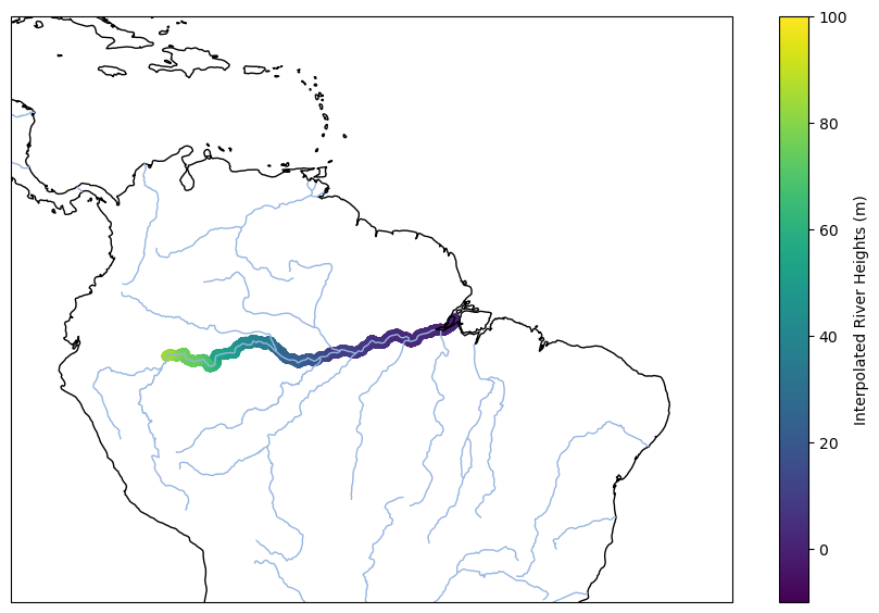

Sea Surface Salinity (Multi-mission: SMAP, Aquarius, SMOS)

The shortname for this dataset is ‘OISSS_L4_multimission_7day_v1’ with the concept ID: C2095055342-POCLOUD. This dataset contains hundreds of granules, so it would be impractical to search and copy all of the URLs in Earthdata Search. Using the shortname, we can access all the files at once in the cloud (1.1 GB data).

sss_results = earthaccess.search_data(short_name="OISSS_L4_multimission_7day_v1")

Granules found: 998

The following cell may take up to around 10 minutes to run due to the size of the dataset

#this line ignores warnings about large chunk sizes
dask.config.set(**{'array.slicing.split_large_chunks': False})

ds_sss = xr.open_mfdataset(earthaccess.open(sss_results),
                           combine='by_coords',
                           mask_and_scale=True,
                           decode_cf=True,
                           chunks='auto',
                           engine='h5netcdf')
ds_sss

 Opening 998 granules, approx size: 0.0 GB

<xarray.Dataset>
Dimensions:                    (longitude: 1440, latitude: 720, time: 998)
Coordinates:
  * longitude                  (longitude) float32 -179.9 -179.6 ... 179.6 179.9
  * latitude                   (latitude) float32 -89.88 -89.62 ... 89.62 89.88
  * time                       (time) datetime64[ns] 2011-08-28 ... 2022-08-02
Data variables:
    sss                        (latitude, longitude, time) float32 dask.array<chunksize=(720, 1440, 1), meta=np.ndarray>
    sss_empirical_uncertainty  (latitude, longitude, time) float32 dask.array<chunksize=(720, 1440, 962), meta=np.ndarray>
    sss_uncertainty            (latitude, longitude, time) float32 dask.array<chunksize=(720, 1440, 1), meta=np.ndarray>
Attributes: (12/42)
    Conventions:                   CF-1.8, ACDD-1.3
    standard_name_vocabulary:      CF Standard Name Table v27
    Title:                         Multi-Mission Optimally Interpolated Sea S...
    Short_Name:                    OISSS_L4_multimission_7d_v1
    Version:                       V1.0
    Processing_Level:              Level 4
    ...                            ...
    geospatial_lat_resolution:     0.25
    geospatial_lat_units:          degrees_north
    geospatial_lon_min:            -180.0
    geospatial_lon_max:            180.0
    geospatial_lon_resolution:     0.25
    geospatial_lon_units:          degrees_east

xarray.Dataset

• Dimensions:
  • longitude: 1440
  • latitude: 720
  • time: 998
• Coordinates: (3)
  • longitude
    (longitude)
    float32
    -179.9 -179.6 ... 179.6 179.9

    long_name :

    longitude

    standard_name :

    longitude

    units :

    degrees_east

    axis :

    X

    valid_min :

    -180.0

    valid_max :

    180.0

    coverage_content_type :

    coordinate

    array([-179.875, -179.625, -179.375, ...,  179.375,  179.625,  179.875],
          dtype=float32)

  • latitude
    (latitude)
    float32
    -89.88 -89.62 ... 89.62 89.88

    long_name :

    latitude

    standard_name :

    latitude

    units :

    degrees_north

    axis :

    Y

    valid_min :

    -90.0

    valid_max :

    90.0

    coverage_content_type :

    coordinate

    array([-89.875, -89.625, -89.375, ...,  89.375,  89.625,  89.875],
          dtype=float32)

  • time
    (time)
    datetime64[ns]
    2011-08-28 ... 2022-08-02

    long_name :

    center day of a time period over which satellite Level 2 SSS data have been collected for OISSS analysis

    standard_name :

    time

    axis :

    T

    coverage_content_type :

    coordinate

    array(['2011-08-28T00:00:00.000000000', '2011-09-01T00:00:00.000000000',
           '2011-09-05T00:00:00.000000000', ..., '2022-07-25T00:00:00.000000000',
           '2022-07-29T00:00:00.000000000', '2022-08-02T00:00:00.000000000'],
          dtype='datetime64[ns]')

• Data variables: (3)
  • sss
    (latitude, longitude, time)
    float32
    dask.array<chunksize=(720, 1440, 1), meta=np.ndarray>

    long_name :

    sea surface salinity

    standard_name :

    sea_surface_salinity

    units :

    1e-3

    valid_min :

    0.0

    valid_max :

    45.0

    add_factor :

    0.0

    coverage_content_type :

    physicalMeasurement

    Array Chunk Bytes 3.85 GiB 150.29 MiB Shape (720, 1440, 998) (720, 1440, 38) Dask graph 961 chunks in 1939 graph layers Data type float32 numpy.ndarray

  • sss_empirical_uncertainty
    (latitude, longitude, time)
    float32
    dask.array<chunksize=(720, 1440, 962), meta=np.ndarray>

    long_name :

    estimated empirical uncertainty of multi-mission OISSS

    units :

    1e-3

    valid_min :

    0.0

    valid_max :

    45.0

    add_factor :

    0.0

    coverage_content_type :

    qualityInformation

    Array Chunk Bytes 3.85 GiB 3.72 GiB Shape (720, 1440, 998) (720, 1440, 962) Dask graph 37 chunks in 86 graph layers Data type float32 numpy.ndarray

  • sss_uncertainty
    (latitude, longitude, time)
    float32
    dask.array<chunksize=(720, 1440, 1), meta=np.ndarray>

    long_name :

    estimated empirical uncertainty of multi-mission OISSS

    units :

    1e-3

    valid_min :

    0.0

    valid_max :

    45.0

    add_factor :

    0.0

    coordinates :

    time longitude latudude

    coverage_content_type :

    qualityInformation

    Array Chunk Bytes 3.85 GiB 150.29 MiB Shape (720, 1440, 998) (720, 1440, 38) Dask graph 961 chunks in 1934 graph layers Data type float32 numpy.ndarray

• Indexes: (3)
  • longitude
    PandasIndex

    PandasIndex(Index([-179.875, -179.625, -179.375, -179.125, -178.875, -178.625, -178.375,
           -178.125, -177.875, -177.625,
           ...
            177.625,  177.875,  178.125,  178.375,  178.625,  178.875,  179.125,
            179.375,  179.625,  179.875],
          dtype='float32', name='longitude', length=1440))

  • latitude
    PandasIndex

    PandasIndex(Index([-89.875, -89.625, -89.375, -89.125, -88.875, -88.625, -88.375, -88.125,
           -87.875, -87.625,
           ...
            87.625,  87.875,  88.125,  88.375,  88.625,  88.875,  89.125,  89.375,
            89.625,  89.875],
          dtype='float32', name='latitude', length=720))

  • time
    PandasIndex

    PandasIndex(DatetimeIndex(['2011-08-28', '2011-09-01', '2011-09-05', '2011-09-09',
                   '2011-09-13', '2011-09-17', '2011-09-21', '2011-09-25',
                   '2011-09-29', '2011-10-03',
                   ...
                   '2022-06-27', '2022-07-01', '2022-07-05', '2022-07-09',
                   '2022-07-13', '2022-07-17', '2022-07-21', '2022-07-25',
                   '2022-07-29', '2022-08-02'],
                  dtype='datetime64[ns]', name='time', length=998, freq=None))

• Attributes: (42)

  Conventions :

  CF-1.8, ACDD-1.3

  standard_name_vocabulary :

  CF Standard Name Table v27

  Title :

  Multi-Mission Optimally Interpolated Sea Surface Salinity 7-Day Global Dataset V1.0

  Short_Name :

  OISSS_L4_multimission_7d_v1

  Version :

  V1.0

  Processing_Level :

  Level 4

  source :

  Aquarius V5.0 Level 2 SSS; SMAP RSS V4.0 Level 2 SSS_40km; SMOS Level 2 SSS L2OS version 662

  sourse_of_input_Aquarius_SSS :

  Aquarius Official Release Level 2 Sea Surface Salinity & Wind Speed Cal Data V5.0. Distributed by PO.DAAC at https://podaac.jpl.nasa.gov/dataset/AQUARIUS_L2_SSS_CAL_V5

  sourse_of_input_SMAP_SSS :

  Meissner, T., F. Wentz, A. Manaster, R. Lindsley, 2019. Remote Sensing Systems SMAP L2C Sea Surface Salinity, Version 4.0 Validated Release, Remote Sensing Systems, Santa Rosa, CA, USA, Available online at www.remss.com/missions/smap.

  sourse_of_input_SMOS_SSS :

  ESA SMOS online dissemination service at https://smos-diss.eo.esa.int/oads/access

  platform :

  Aquarius/SAC-D, SMAP, SMOS

  instrument :

  Aquarius radiometer, SMAP radiometer, SMOS MIRAS

  Creation_Date :

  2023-01-16T04:04:41Z

  Creator_Name :

  Oleg Melnichenko

  Creator_Email :

  oleg@hawaii.edu

  Creator_URL :

  http://iprc.soest.hawaii.edu/users/oleg/oisss/GLB

  Project :

  NASA Ocean Salinity

  Keywords :

  Sea Surface Salinity, SSS, Aquarius, SMAP, Optimum Interpolation, OISSS

  Keywords_vocabulary :

  NASA Global Change Master Directory (GCMD) Science Keywords

  Institution :

  IPRC/SOEST, University of Hawaii, Honolulu, HI; Remote Sensing Systems (RSS), Santa Rosa, CA

  Publisher_Name :

  Oleg Melnichenko, Peter Hacker, James Potemra, Thomas Meissner, Frank Wentz

  Publisher_Email :

  oleg@hawaii.edu.org

  Publisher_URL :

  http://iprc.soest.hawaii.edu/users/oleg/oisss/GLB

  Dataset_Citation_Authors :

  Oleg Melnichenko, Peter Hacker, James Potemra, Thomas Meissner, Frank Wentz

  Dataset_Citation_Year :

  2021

  Dataset_Citation_Product :

  Aquarius/SMAP Sea Surface Salinity Optimum Interpolation Analysis

  Technical_Notes :

  http://iprc.soest.hawaii.edu/users/oleg/oisss/GLB/OISSS_Product_Notes.pdf

  year_of_observation :

  2022

  month_of_observation :

  3

  day_of_observation :

  11

  time_coverage_start :

  2022-03-07T12:00:00Z

  time_coverage_end :

  2022-03-15T12:00:00Z

  time_coverage_resolution :

  P7D

  cdm_data_type :

  grid

  geospatial_lat_min :

  -90.0

  geospatial_lat_max :

  90.0

  geospatial_lat_resolution :

  0.25

  geospatial_lat_units :

  degrees_north

  geospatial_lon_min :

  -180.0

  geospatial_lon_max :

  180.0

  geospatial_lon_resolution :

  0.25

  geospatial_lon_units :

  degrees_east

Plot a subset of the data

Use the function xarray.DataSet.sel to select a subset of the data at the outlet of the Amazon to plot at time t=0 (August 28, 2011) with hvplot.

lat_bnds, lon_bnds = [-2, 6], [-52, -44] 
ds_sss_subset = ds_sss.sel(latitude=slice(*lat_bnds), longitude=slice(*lon_bnds))
ds_sss_subset

ds_sss_subset.sss[:,:,0].hvplot() 

Sea Surface Temperature (MODIS)

MODIS has SST data that coincides with the period used for SSS, 2011-present (943 MB), and has the short name: “MODIS_AQUA_L3_SST_MID-IR_MONTHLY_9KM_NIGHTTIME_V2019.0”. Let’s access this in the same method as before.

Get a list of files so we can open them all at once, creating an xarray dataset using the open_mfdataset() function to “read in” all of the netCDF4 files in one call. MODIS does not have a built-in time variable like SSS, but it is subset by latitude and longitude coordinates. We need to combine the files using the nested format with a created ‘time’ dimension.

modis_results = earthaccess.search_data(short_name="MODIS_AQUA_L3_SST_MID-IR_MONTHLY_9KM_NIGHTTIME_V2019.0", temporal = ("2011-01-01", "2023-01-01"))

Granules found: 143

MODIS did not come with a time variable, so it needs to be extracted from the file names and added in the file preprocessing so files can be successfully concatenated.

#function for time dimension added to each netCDF file
def preprocessing(ds): 
    file_name = ds.product_name
    file_date = basename(file_name).split("_")[2][:6]
    file_date_c = datetime.strptime(file_date, "%Y%m")
    time_point = [file_date_c]
    ds.coords['time'] = ('time', time_point) #expand the dimensions to include time
    return ds

ds_MODIS = xr.open_mfdataset(earthaccess.open(modis_results), combine='by_coords', join='override', mask_and_scale=True, decode_cf=True, chunks='auto',preprocess = preprocessing)
ds_MODIS

 Opening 143 granules, approx size: 0.0 GB

<xarray.Dataset>
Dimensions:    (time: 143, lat: 2160, lon: 4320, rgb: 3, eightbitcolor: 256)
Coordinates:
  * lat        (lat) float32 89.96 89.88 89.79 89.71 ... -89.79 -89.88 -89.96
  * lon        (lon) float32 -180.0 -179.9 -179.8 -179.7 ... 179.8 179.9 180.0
  * time       (time) datetime64[ns] 2011-01-01 2011-02-01 ... 2023-01-01
Dimensions without coordinates: rgb, eightbitcolor
Data variables:
    sst4       (time, lat, lon) float32 dask.array<chunksize=(1, 2160, 4320), meta=np.ndarray>
    qual_sst4  (time, lat, lon) float32 dask.array<chunksize=(1, 2160, 4320), meta=np.ndarray>
    palette    (time, lon, lat, rgb, eightbitcolor) uint8 dask.array<chunksize=(1, 4320, 2160, 3, 256), meta=np.ndarray>
Attributes: (12/59)
    product_name:                     AQUA_MODIS.20110101_20110131.L3m.MO.SST...
    instrument:                       MODIS
    title:                            MODISA Level-3 Standard Mapped Image
    project:                          Ocean Biology Processing Group (NASA/GS...
    platform:                         Aqua
    temporal_range:                   month
    ...                               ...
    publisher_url:                    https://oceandata.sci.gsfc.nasa.gov
    processing_level:                 L3 Mapped
    cdm_data_type:                    grid
    data_bins:                        4834400
    data_minimum:                     -1.635
    data_maximum:                     32.06999

xarray.Dataset

• Dimensions:
  • time: 143
  • lat: 2160
  • lon: 4320
  • rgb: 3
  • eightbitcolor: 256
• Coordinates: (3)
  • lat
    (lat)
    float32
    89.96 89.88 89.79 ... -89.88 -89.96

    long_name :

    Latitude

    units :

    degrees_north

    standard_name :

    latitude

    valid_min :

    -90.0

    valid_max :

    90.0

    array([ 89.958336,  89.875   ,  89.79167 , ..., -89.791664, -89.87501 ,
           -89.958336], dtype=float32)

  • lon
    (lon)
    float32
    -180.0 -179.9 ... 179.9 180.0

    long_name :

    Longitude

    units :

    degrees_east

    standard_name :

    longitude

    valid_min :

    -180.0

    valid_max :

    180.0

    array([-179.95833, -179.875  , -179.79166, ...,  179.79167,  179.87502,
            179.95836], dtype=float32)

  • time
    (time)
    datetime64[ns]
    2011-01-01 ... 2023-01-01

    array(['2011-01-01T00:00:00.000000000', '2011-02-01T00:00:00.000000000',
           '2011-03-01T00:00:00.000000000', '2011-04-01T00:00:00.000000000',
           '2011-05-01T00:00:00.000000000', '2011-06-01T00:00:00.000000000',
           '2011-07-01T00:00:00.000000000', '2011-08-01T00:00:00.000000000',
           '2011-09-01T00:00:00.000000000', '2011-10-01T00:00:00.000000000',
           '2011-11-01T00:00:00.000000000', '2011-12-01T00:00:00.000000000',
           '2012-01-01T00:00:00.000000000', '2012-02-01T00:00:00.000000000',
           '2012-03-01T00:00:00.000000000', '2012-04-01T00:00:00.000000000',
           '2012-05-01T00:00:00.000000000', '2012-06-01T00:00:00.000000000',
           '2012-07-01T00:00:00.000000000', '2012-08-01T00:00:00.000000000',
           '2012-09-01T00:00:00.000000000', '2012-10-01T00:00:00.000000000',
           '2012-11-01T00:00:00.000000000', '2012-12-01T00:00:00.000000000',
           '2013-01-01T00:00:00.000000000', '2013-02-01T00:00:00.000000000',
           '2013-03-01T00:00:00.000000000', '2013-04-01T00:00:00.000000000',
           '2013-05-01T00:00:00.000000000', '2013-06-01T00:00:00.000000000',
           '2013-07-01T00:00:00.000000000', '2013-08-01T00:00:00.000000000',
           '2013-09-01T00:00:00.000000000', '2013-10-01T00:00:00.000000000',
           '2013-11-01T00:00:00.000000000', '2013-12-01T00:00:00.000000000',
           '2014-01-01T00:00:00.000000000', '2014-02-01T00:00:00.000000000',
           '2014-03-01T00:00:00.000000000', '2014-04-01T00:00:00.000000000',
           '2014-05-01T00:00:00.000000000', '2014-06-01T00:00:00.000000000',
           '2014-07-01T00:00:00.000000000', '2014-08-01T00:00:00.000000000',
           '2014-09-01T00:00:00.000000000', '2014-10-01T00:00:00.000000000',
           '2014-11-01T00:00:00.000000000', '2014-12-01T00:00:00.000000000',
           '2015-01-01T00:00:00.000000000', '2015-02-01T00:00:00.000000000',
           '2015-03-01T00:00:00.000000000', '2015-04-01T00:00:00.000000000',
           '2015-05-01T00:00:00.000000000', '2015-06-01T00:00:00.000000000',
           '2015-07-01T00:00:00.000000000', '2015-08-01T00:00:00.000000000',
           '2015-09-01T00:00:00.000000000', '2015-10-01T00:00:00.000000000',
           '2015-11-01T00:00:00.000000000', '2015-12-01T00:00:00.000000000',
           '2016-01-01T00:00:00.000000000', '2016-02-01T00:00:00.000000000',
           '2016-03-01T00:00:00.000000000', '2016-04-01T00:00:00.000000000',
           '2016-05-01T00:00:00.000000000', '2016-06-01T00:00:00.000000000',
           '2016-07-01T00:00:00.000000000', '2016-08-01T00:00:00.000000000',
           '2016-09-01T00:00:00.000000000', '2016-10-01T00:00:00.000000000',
           '2016-11-01T00:00:00.000000000', '2016-12-01T00:00:00.000000000',
           '2017-01-01T00:00:00.000000000', '2017-02-01T00:00:00.000000000',
           '2017-03-01T00:00:00.000000000', '2017-04-01T00:00:00.000000000',
           '2017-05-01T00:00:00.000000000', '2017-06-01T00:00:00.000000000',
           '2017-07-01T00:00:00.000000000', '2017-08-01T00:00:00.000000000',
           '2017-09-01T00:00:00.000000000', '2017-10-01T00:00:00.000000000',
           '2017-11-01T00:00:00.000000000', '2017-12-01T00:00:00.000000000',
           '2018-01-01T00:00:00.000000000', '2018-02-01T00:00:00.000000000',
           '2018-03-01T00:00:00.000000000', '2018-04-01T00:00:00.000000000',
           '2018-05-01T00:00:00.000000000', '2018-06-01T00:00:00.000000000',
           '2018-07-01T00:00:00.000000000', '2018-08-01T00:00:00.000000000',
           '2018-09-01T00:00:00.000000000', '2018-10-01T00:00:00.000000000',
           '2018-11-01T00:00:00.000000000', '2018-12-01T00:00:00.000000000',
           '2019-01-01T00:00:00.000000000', '2019-02-01T00:00:00.000000000',
           '2019-03-01T00:00:00.000000000', '2019-04-01T00:00:00.000000000',
           '2019-05-01T00:00:00.000000000', '2019-06-01T00:00:00.000000000',
           '2019-07-01T00:00:00.000000000', '2019-08-01T00:00:00.000000000',
           '2019-09-01T00:00:00.000000000', '2019-10-01T00:00:00.000000000',
           '2019-11-01T00:00:00.000000000', '2019-12-01T00:00:00.000000000',
           '2020-01-01T00:00:00.000000000', '2020-02-01T00:00:00.000000000',
           '2020-03-01T00:00:00.000000000', '2020-04-01T00:00:00.000000000',
           '2020-05-01T00:00:00.000000000', '2020-06-01T00:00:00.000000000',
           '2020-07-01T00:00:00.000000000', '2020-08-01T00:00:00.000000000',
           '2020-09-01T00:00:00.000000000', '2020-10-01T00:00:00.000000000',
           '2020-11-01T00:00:00.000000000', '2020-12-01T00:00:00.000000000',
           '2021-01-01T00:00:00.000000000', '2021-02-01T00:00:00.000000000',
           '2021-03-01T00:00:00.000000000', '2021-04-01T00:00:00.000000000',
           '2021-05-01T00:00:00.000000000', '2021-06-01T00:00:00.000000000',
           '2021-07-01T00:00:00.000000000', '2021-09-01T00:00:00.000000000',
           '2021-10-01T00:00:00.000000000', '2021-11-01T00:00:00.000000000',
           '2021-12-01T00:00:00.000000000', '2022-01-01T00:00:00.000000000',
           '2022-02-01T00:00:00.000000000', '2022-03-01T00:00:00.000000000',
           '2022-04-01T00:00:00.000000000', '2022-05-01T00:00:00.000000000',
           '2022-06-01T00:00:00.000000000', '2022-07-01T00:00:00.000000000',
           '2022-08-01T00:00:00.000000000', '2022-09-01T00:00:00.000000000',
           '2022-10-01T00:00:00.000000000', '2022-11-01T00:00:00.000000000',
           '2023-01-01T00:00:00.000000000'], dtype='datetime64[ns]')

• Data variables: (3)
  • sst4
    (time, lat, lon)
    float32
    dask.array<chunksize=(1, 2160, 4320), meta=np.ndarray>

    long_name :

    4um Sea Surface Temperature

    units :

    degree_C

    standard_name :

    sea_surface_temperature

    valid_min :

    -1000

    valid_max :

    10000

    display_scale :

    linear

    display_min :

    -2.0

    display_max :

    45.0

    Array Chunk Bytes 4.97 GiB 35.60 MiB Shape (143, 2160, 4320) (1, 2160, 4320) Dask graph 143 chunks in 430 graph layers Data type float32 numpy.ndarray

  • qual_sst4
    (time, lat, lon)
    float32
    dask.array<chunksize=(1, 2160, 4320), meta=np.ndarray>

    long_name :

    Quality Levels, Sea Surface Temperature

    valid_min :

    0

    valid_max :

    5

    Array Chunk Bytes 4.97 GiB 35.60 MiB Shape (143, 2160, 4320) (1, 2160, 4320) Dask graph 143 chunks in 430 graph layers Data type float32 numpy.ndarray

  • palette
    (time, lon, lat, rgb, eightbitcolor)
    uint8
    dask.array<chunksize=(1, 4320, 2160, 3, 256), meta=np.ndarray>

    Array Chunk Bytes 0.93 TiB 6.67 GiB Shape (143, 4320, 2160, 3, 256) (1, 4320, 2160, 3, 256) Dask graph 143 chunks in 716 graph layers Data type uint8 numpy.ndarray

• Indexes: (3)
  • lat
    PandasIndex

    PandasIndex(Index([ 89.95833587646484,             89.875,  89.79167175292969,
            89.70833587646484,             89.625,  89.54167175292969,
            89.45833587646484,             89.375,  89.29167175292969,
            89.20833587646484,
           ...
           -89.20833587646484, -89.29166412353516, -89.37500762939453,
           -89.45833587646484, -89.54166412353516, -89.62500762939453,
           -89.70833587646484, -89.79166412353516, -89.87500762939453,
           -89.95833587646484],
          dtype='float32', name='lat', length=2160))

  • lon
    PandasIndex

    PandasIndex(Index([ -179.9583282470703,            -179.875, -179.79165649414062,
            -179.7083282470703,            -179.625, -179.54165649414062,
            -179.4583282470703,            -179.375, -179.29165649414062,
            -179.2083282470703,
           ...
            179.20835876464844,   179.2916717529297,  179.37501525878906,
            179.45835876464844,   179.5416717529297,  179.62501525878906,
            179.70835876464844,   179.7916717529297,  179.87501525878906,
            179.95835876464844],
          dtype='float32', name='lon', length=4320))

  • time
    PandasIndex

    PandasIndex(DatetimeIndex(['2011-01-01', '2011-02-01', '2011-03-01', '2011-04-01',
                   '2011-05-01', '2011-06-01', '2011-07-01', '2011-08-01',
                   '2011-09-01', '2011-10-01',
                   ...
                   '2022-03-01', '2022-04-01', '2022-05-01', '2022-06-01',
                   '2022-07-01', '2022-08-01', '2022-09-01', '2022-10-01',
                   '2022-11-01', '2023-01-01'],
                  dtype='datetime64[ns]', name='time', length=143, freq=None))

• Attributes: (59)

  product_name :

  AQUA_MODIS.20110101_20110131.L3m.MO.SST4.sst4.9km.nc

  instrument :

  MODIS

  title :

  MODISA Level-3 Standard Mapped Image

  project :

  Ocean Biology Processing Group (NASA/GSFC/OBPG)

  platform :

  Aqua

  temporal_range :

  month

  processing_version :

  R2019.0

  date_created :

  2019-12-17T18:28:57.000Z

  history :

  l3mapgen par=AQUA_MODIS.20110101_20110131.L3m.MO.SST4.sst4.9km.nc.param

  l2_flag_names :

  LAND,~HISOLZEN

  time_coverage_start :

  2010-12-31T12:10:01.000Z

  time_coverage_end :

  2011-01-31T14:29:59.000Z

  start_orbit_number :

  46065

  end_orbit_number :

  46518

  map_projection :

  Equidistant Cylindrical

  latitude_units :

  degrees_north

  longitude_units :

  degrees_east

  northernmost_latitude :

  90.0

  southernmost_latitude :

  -90.0

  westernmost_longitude :

  -180.0

  easternmost_longitude :

  180.0

  geospatial_lat_max :

  90.0

  geospatial_lat_min :

  -90.0

  geospatial_lon_max :

  180.0

  geospatial_lon_min :

  -180.0

  latitude_step :

  0.083333336

  longitude_step :

  0.083333336

  sw_point_latitude :

  -89.958336

  sw_point_longitude :

  -179.95833

  spatialResolution :

  9.28 km

  geospatial_lon_resolution :

  0.083333336

  geospatial_lat_resolution :

  0.083333336

  geospatial_lat_units :

  degrees_north

  geospatial_lon_units :

  degrees_east

  number_of_lines :

  2160

  number_of_columns :

  4320

  measure :

  Mean

  suggested_image_scaling_minimum :

  -2.0

  suggested_image_scaling_maximum :

  45.0

  suggested_image_scaling_type :

  LINEAR

  suggested_image_scaling_applied :

  No

  _lastModified :

  2019-12-17T18:28:57.000Z

  Conventions :

  CF-1.6 ACDD-1.3

  institution :

  NASA Goddard Space Flight Center, Ocean Ecology Laboratory, Ocean Biology Processing Group

  standard_name_vocabulary :

  CF Standard Name Table v36

  naming_authority :

  gov.nasa.gsfc.sci.oceandata

  id :

  AQUA_MODIS.20110101_20110131.L3b.MO.SST4.nc/L3/AQUA_MODIS.20110101_20110131.L3b.MO.SST4.nc

  license :

  https://science.nasa.gov/earth-science/earth-science-data/data-information-policy/

  creator_name :

  NASA/GSFC/OBPG

  publisher_name :

  NASA/GSFC/OBPG

  creator_email :

  data@oceancolor.gsfc.nasa.gov

  publisher_email :

  data@oceancolor.gsfc.nasa.gov

  creator_url :

  https://oceandata.sci.gsfc.nasa.gov

  publisher_url :

  https://oceandata.sci.gsfc.nasa.gov

  processing_level :

  L3 Mapped

  cdm_data_type :

  grid

  data_bins :

  4834400

  data_minimum :

  -1.635

  data_maximum :

  32.06999

Plot a subset of the data

Use the function xarray.DataSet.sel to select a subset of the data at the outlet of the Amazon to plot with hvplot.

lat_bnds, lon_bnds = [6,-2], [-52, -44] 
ds_MODIS_subset = ds_MODIS.sel(lat=slice(*lat_bnds), lon=slice(*lon_bnds))
ds_MODIS_subset

ds_MODIS_subset.sst4.hvplot.image(y='lat', x='lon', cmap='viridis').opts(clim=(22,30))

Time Series Comparison

Plot each dataset for the time period 2011-2019.

First, we need to average all pixels in the subset lat/lon per time for sea surface salinity and sea surface temperature to set up for the graphs.

sss_mean = []
for t in np.arange(len(ds_sss_subset.time)):
    sss_mean.append(np.nanmean(ds_sss_subset.sss[:,:,t].values))

#sss_mean

#MODIS
sst_MODIS_mean = []
for t in np.arange(len(ds_MODIS_subset.time)):
    sst_MODIS_mean.append(np.nanmean(ds_MODIS_subset.sst4[t,:,:].values))
    
#sst_MODIS_mean

Combined timeseries plot of river height and LWE thickness

Both datasets are mapped for the outlet of the Amazon River into the estuary.

#plot river height and land water equivalent thickness
fig, ax1 = plt.subplots(figsize=[12,7])

#plot river height
ds_MEaSUREs.height[16,6689:9469].plot(color='darkblue')

#plot LWE thickness on secondary axis
ax2 = ax1.twinx()
ax2.plot(ds_GRACE_subset.time[107:179], ds_GRACE_subset.lwe_thickness[107:179,34,69], color = 'darkorange')

ax1.set_xlabel('Date')
ax2.set_ylabel('Land Water Equivalent Thickness (cm)', color='darkorange')
ax1.set_ylabel('River Height (m)', color='darkblue')
ax2.legend(['GRACE-FO'], loc='upper right')
ax1.legend(['Pre-SWOT MEaSUREs'], loc='lower right')

plt.title('Amazon Estuary, 2011-2019 Lat, Lon = (-0.7, -50)')
ax1.grid()
plt.show()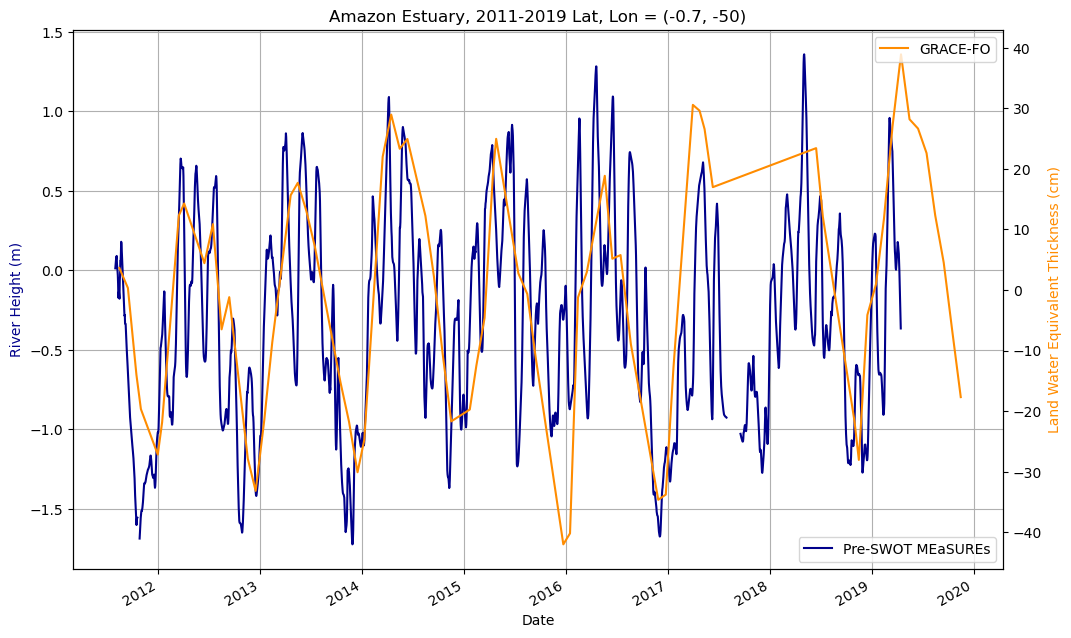

LWE thickness captures the seasonality of Pre-SWOT MEaSUREs river heights well, and so LWE thickness can be compared to all other variables as a representative of the seasonality of both measurements for the purpose of this notebook.

Combined timeseries plots of salinity and LWE thickness, followed by temperature

#Combined Subplots
fig = plt.figure(figsize=(10,10))

ax1 = fig.add_subplot(211)
plt.title('Amazon Estuary, 2011-2019')
ax2 = ax1.twinx()
ax3 = plt.subplot(212)
ax4 = ax3.twinx()

#lwe thickness
ax1.plot(ds_GRACE_subset.time[107:179], ds_GRACE_subset.lwe_thickness[107:179,34,69], color = 'darkorange')
ax1.set_ylabel('LWE Thickness (cm)', color='darkorange')
ax1.grid()

#sea surface salinity
ax2.plot(ds_sss_subset.time[0:750], sss_mean[0:750], 'g')
ax2.set_ylabel('SSS (psu)', color='g')

#sea surface temperature
ax3.plot(ds_MODIS_subset.time[7:108], sst_MODIS_mean[7:108], 'darkred')
ax3.set_ylabel('SST (deg C)', color='darkred')
ax3.grid()

#river height at outlet
ds_MEaSUREs.height[16,6689:9469].plot(color='darkblue')
ax4.set_ylabel('River Height (m)', color='darkblue')

Text(0, 0.5, 'River Height (m)')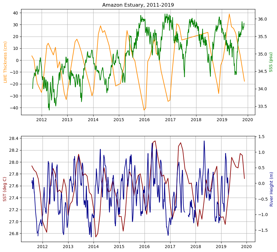

Measurements of LWE thickness and SSS follow expected patterns. When lwe thickness is at its lowest, indicating less water is flowing through during the drought, salinity is at its highest. Without high volume of water pouring into the estuary, salinity increases. We can see that temperature is shifted a bit in time from river height as well at the outlet, a relationship that could be further explored.