Earthdata Webinar

imported on: 2024-04-15

This notebook is from a different repository in NASA’s PO.DAAC, the-coding-club

The original source for this document is https://github.com/podaac/the-coding-club/blob/main/notebooks/Earthdata_webinar_20220727.ipynb

Disclaimer: Reference herein to any specific commercial product, process, or service by trade name, trademark, manufacturer, or otherwise, does not constitute or imply its endorsement by the United States Government or the Jet Propulsion Laboratory, California Institute of Technology.

Moving Code to the Data: Analyzing Sea Level Rise Using Earth Data in the Cloud

Jinbo Wang Jinbo.Wang@jpl.nasa.gov, Ed Armstrong, Ian Fenty, Nikki Tebaldi, Jack McNeils, Jonathan Smolenski, Stepheny Perez, Catalina Oaida, Mike Gangl

PO.DAAC, Jet Propulsion Laboratory, California Institution of Technology

Earthdata Webinar, July 27, 2022

Ackowledgement: PO.DAAC coding club team, Openscapes, NASA Earthdata EOSDIS

This note book was created for the Earthdata webinar. The webinar recording is available on NASA’s Earthdata youtube channel and embeded below.

%%html
<iframe width="560" height="315" src="https://www.youtube.com/embed/4BcoLh8vMG4" title="YouTube video player" frameborder="0" allow="accelerometer; autoplay; clipboard-write; encrypted-media; gyroscope; picture-in-picture" allowfullscreen></iframe>

Abstract

Nearly a petabyte of NASA’s Physical Oceanography Distributed Active Archive Center (PO.DAAC) data products have been moved to NASA’s Earthdata Cloud—hosted in the Amazon Web Services (AWS) cloud. To maximize the full potential of cloud computing on the big Data, one needs to be familiar with not only the data products and their access methods, but also a new set of knowledge for working in a cloud environment. This can be a daunting task for the majority of the science community, who may be familiar with high-performance computing, but not with AWS services. To aid end users in learning and to be successful during this paradigm shift, the PO.DAAC team has been exploring pathways toward practical solutions to help research groups migrate their workflow into cloud.
During this webinar we will explain basic concepts of working in the cloud and use a simple science use case to demonstrate the workflow. Participants do not need prior knowledge of AWS services and the Earthdata Cloud. This is a step-by-step walkthrough of exploring and discovering PO.DAAC data and applying AWS cloud computing to analyze global sea level rise from altimetry data and Estimating the Circulation and Climate of the Ocean (ECCO) products.
We hope that you can start to practice cloud computing using AWS and PODAAC/Earthdata cloud products by following the 6 steps in this tutorial without investing a large amount of time.

Motivation

It is expected the NASA Earthdata will grow to >250 PB in 2025,
Cloud computing has a big potential
The path to the cloud computing is unclear for majority of the science and application community
The science community are often perplexed at the start line by a new language related to cloud computing and the large amount of different AWS tools and services, such as CloudFront, EC2, VPC, AMI, IAM, Bucket, Glacier, Snowcone, Snowball, Snowmobile, data lakes, just to name a few.
We aim to share our experience of passing the start line and start to run cloud computing, demonstrate a use case assuming zero knowledge of AWS cloud
The global mean sea level used here is an important climate indicator and relatively easy to calculate from the PODAAC data in the cloud.

Objectives

Set up a cloud computing environment from scrath
Run the global mean sea level code in the cloud
Build a webpage server using the same cloud computer

Target audience

Science- and application-oriented group who
- has interest in cloud computing;
- is familiar with python, conda, and jupyter-notebook;
- but with limited knowledge of NASA Earthdata and IT;
- and zero knowledge of AWS cloud. *** ## Outline: the steps toward running in-cloud analysis

Get an AWS account
Start an AWS cloud computer (Elastic Computer Cloud, EC2)
1. explain AWS console, EC2 instance
Configure the EC2 with the necessary software
1. While waiting, explain the global mean sea level analysis code
Configure a jupyter-lab on the EC2 and connect to it from browser
Demo the code (this notebook) in the cloud and save the figure
Set up an apache server (hosting website)
- Create a static html webpage to show the result

There are many ways to achieve this goal. Many alternatives are much smarter but they usually involves a set of new knowledge related to cloud and/or AWS that steepens the learning curve and sometimes makes the process intimidating. The following steps are suggested here because it is believed to involve a minimum amount of specilized knowledge beyond our common practice on our own computer.

Important terms

AWS terminology	Long name	Meaning
AWS Region		AWS facility. There are many of them. NASA Earth Data are in US-WEST-2, somewhere in Oregon.
EC2	Elastic Computer Cloud	A computer in one of the AWS regions. It is a common practice that you should use an EC2 in the region where you data is hosted.
AWS console		A web-based control panel for all AWS tools and services. You can start an EC2, create a storage disk (S3 bucket) and much more.
Key Pair		An SSH key generated for accessing the EC2, e.g., through SSH. Anyone who has your key can connect to your EC2. It means that you can share the same EC2 with others just through sharing a Key Pair file.

Step 1 – Get an AWS account

If you already have an AWS account, skip to Step 2. ### Choices: 1. Look for institutional support (recommended) 1. Engage in NASA-funded programs (e.g., openscapes) 1. Apply a free AWS account (today’s focus) 1. It is free for a year but only offers small computers (1 CPU, 1GB memory) 1. With the offer of 750 hours per month, a free-tier EC2 can be on all time for a year. 1. Need your personal information including credit card

(https://aws.amazon.com)

This page explains the five steps to create an AWS account. > https://progressivecoder.com/creating-an-aws-account-a-step-by-step-process-guide/. ***

Step 2 - Start an EC2

Log in through aws console https://aws.amazon.com/console/
Start an EC2 (AWS jargon: launch an instance, layman’s interpretation: start a remote server hosted by AWS)
- Name and Tags: earthdata_webinar
- Application and OS Images (Amazon Machine Image): >Red Hat Enterprise Linux 8 (HVM) SSD Volume type (free-tier elegible)
- Instance type: t2.micro (1CPU, 1Gb memory) (If you have a institution- or project-supported AWS account, try to use a bigger computer with >4G memory.)
- Key pair (login): “Create new key pair”
  - enter a name, e.g., “aws_ec2_jupyter” -> create key pair
  - look for the .pem file in the Download folder, move it to .ssh folder. > mv ~/Downloads/aws_ec2_jupyter.pem .ssh/
  - change permission to 400 using > chmod 400 aws_ec2_jupyter.pem
- check the two boxes for HTTP and HTTPS for the webserver
- Add storage: 10 Gb should be fine for prototyping and testing. You have total 30Gb free storage, which can be split among three EC2s for example.
- Click “Launch Instance” button

Reference

AWS get set up for amazon EC2: https://docs.aws.amazon.com/AWSEC2/latest/UserGuide/get-set-up-for-amazon-ec2.html
AWS Get started with AWS EC2: https://docs.aws.amazon.com/AWSEC2/latest/UserGuide/EC2_GetStarted.html ***

Step 3 - Login and install the necessary software and prepare EarthData Login (.netrc)

Find the public IP from your EC2 dashboard. (The EC2 dashboard example: link)
First connect to the instance via ssh.

     ssh -i "~/.ssh/aws_ec2_jupyter.pem" ec2-user@The_public_ip_address -L 9889:localhost:9889

Remember to set the following parameters appropriately: * -i points the ssh client on your local machine at your pem key to authenticate * -L tunnels traffic on port 9889 between the ec2 instance and your local machine. This port number can be any value between 1024 and 32767. 1. Update packages. Optionally install wget, git etc. for downloading this notebook from github.com

 > ```sudo yum update -y && sudo yum install wget -y```

Download miniconda install script into tmp/ and execute it with bash. Then, activate the base environment.

  mkdir -p tmp
  wget https://repo.anaconda.com/miniconda/Miniconda3-latest-Linux-x86_64.sh -O tmp/miniconda.sh && \
  bash tmp/miniconda.sh -b -p $HOME/conda && \
  source ~/conda/bin/activate

Create a new environment called jupyter running Python 3.7; activate it; install JupyterLab and other required packages.

  conda create -n jupyter python=3.7 -y && \
  conda activate jupyter && \
  conda install requests tqdm numpy pandas -y && \
  conda install matplotlib netCDF4 -y &&\
  conda install xarray jupyterlab s3fs hdf5 scipy -y &&\
  conda install pyproj -y

Warning: the free-tier EC2 has only 1Gb memory. Make sure to monitor the installation to avoid memory errors. If the installation is aborted due to lack of memory, repeat the installation again to pass the problem or considering install the packages one by one.

An EarthData Login (EDL) account is needed for accessing NASA Eartdata regardless the location of the data, either in the Earthdata cloud or on-premise from DAACs.
1. Run the following line in the EC2 terminal: >bash echo "machine urs.earthdata.nasa.gov\n login your_earthdata_username\n password your_earthdata_account_password" > ~/.netrc
2. Use a text editor to replace your_earthdata_username with your EDL username and your_earthdata_account_password with your EDL password. > shell vi ~/.netrc
3. Change .netrc file permission: >shell chmod 400 ~/.netrc *** ### Advanced approach using “User data” box to install softwares while launching the EC2 (replacing step 3.3)

The following replaces step 3.3, but is not required in this tutorial.

The system software updates can be done by inserting the following bash script into the “User data” box during the Launch Instance step (Step 2). It replaces Steps 3.3.

#!/bin/bash
  sudo yum update -y
  sudo yum install wget -y
  sudo yum install httpd -y
  sudo service httpd start

Step 4 - Set up a jupyter-lab

Jupyterlab is a web-based interactive development environment for python and other languages. It is a perfect tool for accessing the computing resources on an EC2 through SSH tunneling. Jupyterlab and the associated software are install in Step 3. Here is two steps to start and connect to a jupyterlab server on the EC2.

Use Python to generate and store a hashed password as a shell variable: >

PW="$(python3 -c 'from notebook.auth import passwd; import getpass; print(passwd(getpass.getpass(), algorithm="sha256"))')"

Start jupyter lab instance with the following parameters: >

jupyter lab --port=9889 --ip='127.0.0.1' --NotebookApp.token='' --NotebookApp.password="$PW" --notebook-dir="$HOME" --no-browser```

1. Access the server through your web browser: http://127.0.0.1:9889/

<div class="alert alert-block alert-success">
<b>Optional for convinence</b> </br> 
You can use tmux to start a screen to keep the jupyterlab running on the EC2 even after logging.</br> 

Detach the screen by pressing CTRL + b -> d. 
</div>


#### Reference

* https://jupyterlab.readthedocs.io/en/stable/getting_started/installation.html#conda
* https://requests.readthedocs.io/en/master/user/install/
* https://matplotlib.org/stable/#installation
* https://shapely.readthedocs.io/en/latest/
***

## Step 5 - Run the code (this notebook) in the cloud and save the figure

## Data products

1. MEaSURES-SSH version JPL1812
   - short name: ```SEA_SURFACE_HEIGHT_ALT_GRIDS_L4_2SATS_5DAY_6THDEG_V_JPL1812```
   - [landing page](https://podaac.jpl.nasa.gov/dataset/SEA_SURFACE_HEIGHT_ALT_GRIDS_L4_2SATS_5DAY_6THDEG_V_JPL1812) (Newer version is available)
1. GMSL
   - short name: ```JPL_RECON_GMSL```
   - [landing page](https://podaac.jpl.nasa.gov/dataset/JPL_RECON_GMSL)
1. ECCO global mean sea level (used in the reader's exercise)
   - short name: `ECCO_L4_GMSL_TIME_SERIES_MONTHLY_V4R4`
   - [landing page](https://doi.org/10.5067/ECTSM-MSL44)

::: {#cell-11 .cell execution_count=28}
``` {.python .cell-code}
#load python modules

import xarray as xr
import numpy as np
import pylab as plt
import pandas as pd
#Short_name is used to identify a specific dataset in NASA Earthdata. 
short_name='SEA_SURFACE_HEIGHT_ALT_GRIDS_L4_2SATS_5DAY_6THDEG_V_JPL1812'

:::

The interface to the AWS Simple Storage Service (S3) file system (stores all NASA Earthdata)

PO.DAAC cloud (POCLOUD) is a part of Earthdata Cloud. The data are hosted in a S3 bucket on AWS US-West-2. “US-West-2” is a term that refers to the AWS center in Oregon. In this case, the so-called ‘Direct-S3 access’ only works on the machines hosted in the US-West-2.

s3fs is a pythonic file interface to S3 built on top of botocore. s3fs allows typical file-system style operations like cp, mv, ls, du, glob, and put/get of local files to/from S3. Details can be find on its website https://s3fs.readthedocs.io/en/latest/.

It is important that you set up the .netrc file correctly in order to enable the following init_S3FileSystem module. The .netrc file should be placed in your home folder. A typical .netrc file has the following content:

machine urs.earthdata.nasa.gov
    login your_earthdata_username
    password your_earthdata_account_password

Make sure the permission of the .netrc file is set to 400: chmod 400 ~/.netrc

If you do not have or do not remember your Earthdata Login information, go here to register or here to reset password.

AWS credentials with EDL

AWS requires security credentials to access AWS S3.

With your EDL, you can obtain a temporay S3 credential through https://archive.podaac.earthdata.nasa.gov/s3credentials. It is a ‘digital key’ to access the Earthdata in AWS cloud. Here is an example:

{“accessKeyId”: “xxxx”, “secretAccessKey”: “xxxx”, “sessionToken”: “xxxx”, “expiration”: “2022-07-22 15:56:34+00:00”}

Further reading: https://docs.aws.amazon.com/general/latest/gr/aws-sec-cred-types.html

def init_S3FileSystem():
    """
    This routine automatically pull your EDL crediential from .netrc file and use it to obtain an AWS S3 credential through a podaac service accessable at https://archive.podaac.earthdata.nasa.gov/s3credentials
    
    Return:
    =======
    
    s3: an AWS S3 filesystem
    """
    import requests,s3fs
    creds = requests.get('https://archive.podaac.earthdata.nasa.gov/s3credentials').json()
    s3 = s3fs.S3FileSystem(anon=False,
                           key=creds['accessKeyId'],
                           secret=creds['secretAccessKey'], 
                           token=creds['sessionToken'])
    return s3

Use s3fs.glob to get all file names

The S3FileSystem allows typical file-system style operations like cp, mv, ls, du, glob. Once the s3fs file system is established, we can use ‘glob’ to get all file names from a collection. In this case, the collection S3 path is

s3://podaac-ops-cumulus-protected/SEA_SURFACE_HEIGHT_ALT_GRIDS_L4_2SATS_5DAY_6THDEG_V_JPL1812/

Using the following will get a list netcdf filenames:

fns=s3sys.glob("s3://podaac-ops-cumulus-protected/SEA_SURFACE_HEIGHT_ALT_GRIDS_L4_2SATS_5DAY_6THDEG_V_JPL1812/*.nc")

s3sys=init_S3FileSystem()

s3path="s3://podaac-ops-cumulus-protected/%s/"%short_name
fns=s3sys.glob(s3path+"*.nc")
print(fns[0])
#Set the time stamps associated with the files
time=pd.date_range(start='1992-10-02',periods=len(fns),freq='5D')

podaac-ops-cumulus-protected/SEA_SURFACE_HEIGHT_ALT_GRIDS_L4_2SATS_5DAY_6THDEG_V_JPL1812/ssh_grids_v1812_1992100212.nc

print('There are %i files.'%len(fns))

There are 1922 files.

Here is an example file.

d=xr.open_dataset(s3sys.open(fns[0]))
d

Plot an example

plt.figure(figsize=(15,7))
plt.contourf(d['Longitude'],d['Latitude'],d['SLA'][0,...].T,levels=np.arange(-0.5,0.6,0.05))
plt.ylabel('Latitude')
plt.xlabel('Longitude')
plt.title('Sea Level Anomaly %s'%d.time_coverage_start)

Text(0.5, 1.0, 'Sea Level Anomaly 1992-10-02')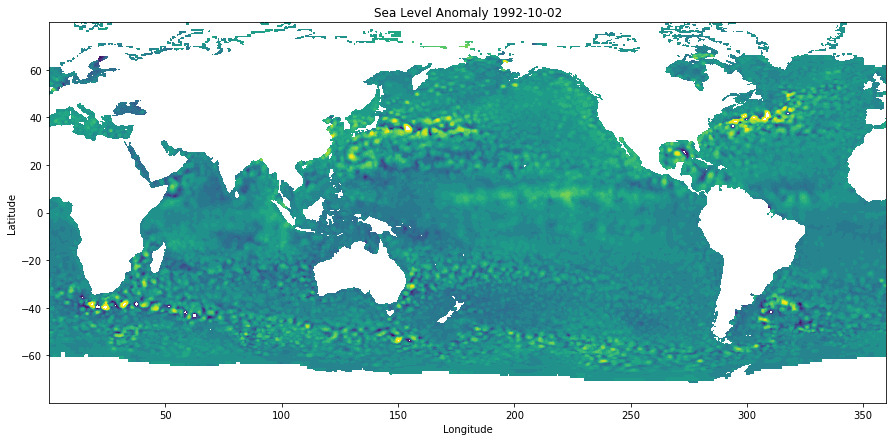

Calculate the global mean SSHA

The global mean SSH is calculated as follows.

\(SSH_{mean} = \sum \eta(\phi,\lambda)*A(\phi)\), where \(\phi\) is latitude, \(\lambda\) is longitude, \(A\) is the area of the grid at latitude \(\phi\), and \(\eta(\phi,\lambda)*A(\phi)\) is the weighted SLA at \((\phi,\lambda)\).

The following routine area pre-calculates the area as a function of latitude for the 1/6-degree resolution grids.

def area(lats):
    """
    Calculate the area associated with a 1/6 by 1/6 degree box at latitude specified in 'lats'. 
    
    Parameter
    ==========
    lats: a list or numpy array of size N
          the latitudes of interest. 
    
    Return
    =======
    out: Array (N)
         area values (unit: m^2)
    """
    # Modules:
    from pyproj import Geod
    # Define WGS84 as CRS:
    geod = Geod(ellps='WGS84')
    dx=1/12.0
    c_area=lambda lat: geod.polygon_area_perimeter(np.r_[-dx,dx,dx,-dx], lat+np.r_[-dx,-dx,dx,dx])[0]
    out=[]
    for lat in lats:
        out.append(c_area(lat))
    return np.array(out)

def global_mean(fn_s3,s3sys,ssh_area):
    """
    Calculate the global mean given an s3 file of SSH, a s3fs.S3FileSystem, 
    and the ssh_area, which is precalculated to save computing time. 
    Parameter:
    ===========
    fn_s3: S3 file name, e.g., s3://podaac-ops-cumulus-protected/SEA_SURFACE_HEIGHT_ALT_GRIDS_L4_2SATS_5DAY_6THDEG_V_JPL1812/ssh_grids_v1812_1992100212.nc
    s3sys: generated by s3fs.S3FileSystem
    ssh_area: the area size associated with MEaSURES-SSH 1/6-degree resolution product. 
    
    Return
    =======
    dout: scalar
          The global mean sea level (default unit from MEaSURES-SSH: meter)
    """
    with xr.open_dataset(s3sys.open(fn_s3))['SLA'] as d:
        dout=((d*ssh_area).sum()/(d/d*ssh_area).sum()).values
    return dout

d=xr.open_dataset(s3sys.open(fns[0]))
#pre-calculate the area for reuse
ssh_area=area(d.Latitude.data).reshape(1,-1)

print('The global mean sea level from %s is %7.5f meters.'%(fns[0],global_mean(fns[0],s3sys,ssh_area) ) )

The global mean sea level from podaac-ops-cumulus-protected/SEA_SURFACE_HEIGHT_ALT_GRIDS_L4_2SATS_5DAY_6THDEG_V_JPL1812/ssh_grids_v1812_1992100212.nc is -0.00632 meters.

Demonstrate using a single thread

Benchmark: using a single thread takes about 17 min to calculate all 1922 files. Here the program is sped up by skipping every 360 days (72 steps). The small EC2 can handle the computation because it involves one file per step.

%%time

#Loop 26-year 5-daily SSH fields (1922 files)
#Skip every 72 files to speed up

result=[]
t_local=time[::72]
for fn in fns[::72]:
    result.append(global_mean(fn,s3sys,ssh_area)*1e3 )
result=np.array(result)

CPU times: user 4.35 s, sys: 1.26 s, total: 5.61 s
Wall time: 45 s

from scipy.stats import linregress

plt.figure(figsize=(14,5))
plt.plot(t_local,result-10,'r-o')
tyr=(t_local-t_local[0])/np.timedelta64(1,'Y') #convert the number of years
msk=np.isnan(result)
tyr=tyr[~msk]
result=result[~msk]

#Calculate the linear trend using linear regression `linregress`
rate=linregress(tyr[1:],result[1:]) 
print('The estimated sea level rise rate between 1993 and 2018: %5.1fmm/year.'%(rate[0]) )
plt.text(t_local[0],10, 'Linear trend: %5.1fmm/year'%(rate[0]),fontsize=16)
plt.xlabel('Time (year)',fontsize=16)
plt.ylabel('Global Mean SLA (mm)',fontsize=16)

plt.grid(True)
plt.show()

The estimated sea level rise rate between 1993 and 2018:   2.5mm/year.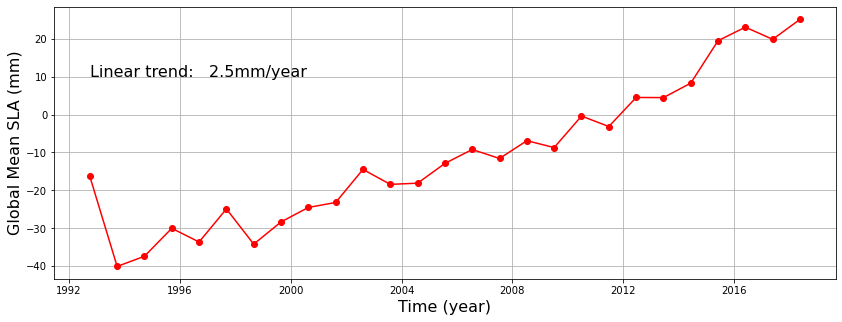

Quiz
The global sea level trend from altimetry should be 3.0mm/year. Why did we get 2.5mm/year from the above analysis? Can you get 3.0mm/year by modifying the above code?

Hint: The above analysis is aliased.

Add the GMSL from Frederikse et al. https://podaac.jpl.nasa.gov/dataset/JPL_RECON_GMSL

from scipy.stats import linregress

plt.figure(figsize=(14,5))
plt.plot(t_local,result-10,'r-o',label='altimetry')

plt.xlabel('Time (year)',fontsize=16)
plt.ylabel('Global Mean SLA (meter)',fontsize=16)
plt.grid(True)

# Add GMSL from 

d1=xr.open_dataset('https://opendap.jpl.nasa.gov/opendap/allData/homage/L4/gmsl/global_timeseries_measures.nc')
print(d1)
d1['global_average_sea_level_change'].plot(label='in-situ')
plt.legend()

plt.savefig('gmsl.png')

<xarray.Dataset>
Dimensions:                                             (time: 119)
Coordinates:
  * time                                                (time) datetime64[ns] ...
Data variables: (12/21)
    global_average_sea_level_change                     (time) float32 ...
    global_average_sea_level_change_upper               (time) float32 ...
    global_average_sea_level_change_lower               (time) float32 ...
    glac_mean                                           (time) float32 ...
    glac_upper                                          (time) float32 ...
    glac_lower                                          (time) float32 ...
    ...                                                  ...
    global_average_thermosteric_sea_level_change        (time) float32 ...
    global_average_thermosteric_sea_level_change_upper  (time) float32 ...
    global_average_thermosteric_sea_level_change_lower  (time) float32 ...
    sum_of_contrib_processes_mean                       (time) float32 ...
    sum_of_contrib_processes_upper                      (time) float32 ...
    sum_of_contrib_processes_lower                      (time) float32 ...
Attributes: (12/42)
    title:                     Global sea-level changes and contributing proc...
    summary:                   This file contains reconstructed global-mean s...
    id:                        10.5067/GMSLT-FJPL1
    naming_authority:          gov.nasa.jpl
    source:                    Frederikse et al. The causes of sea-level rise...
    project:                   NASA sea-level change science team (N-SLCT)
    ...                        ...
    time_coverage_start:       1900-01-01
    time_coverage_end:         2018-12-31
    time_coverage_duration:    P119Y
    time_coverage_resolution:  P1Y
    date_created:              2020-07-28
    date_modified:             2020-09-14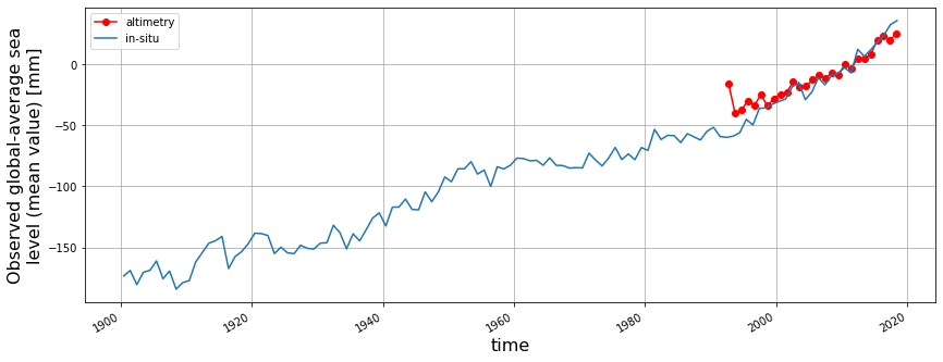

Quiz
The global sea level trend from tide-gauge reconstruction (3.5mm/year) is steeper than altimetry-based analysis (3.0mm/year). Why is that?

Hint: Altimetry-based analysis does not consider vertical land motion.

Step 6 – Run an apache web server to show the result

Because the EC2 was set up to allow HTTPS traffic, we can setup a simple website to host the GMSL result. This simple website should be an illustration using an EC2 to streamline a web application. You can set up a cron job to establish auto-update of the result.

From your EC2 command line, install apache webserver:

sudo yum install httpd -y

Start the server and auto-start when stopped

sudo service httpd start

Copy and paste the following code to make a webpage index.html

<html>
<head>
    <center>
     <h1 style="font-size:30px">The global mean sea level </h1>
     <h2 style="font-size:20px">Hosted on my personal AWS EC2</h2>
     <img src="gmsl.png" alt="Global Mean Sea Level" width="700">
     <h1 style="font-size:20px">Diagnosed from MEaSURES-SSH (red) and JPL_RECON_GMSL (blue)</h1>
     <h1 style="font-size:20px">Earthdata webinar, 07/27/2022</h1>
     <h1 style="font-size:20px;color=purple">Cloud-based analysis is fun!</h1>
     <img src="https://chucktownfloods.cofc.edu/wp-content/uploads/2019/07/Earthdata-Logo.jpg" width="200">
    </center>
</head>
</html>

Move index.html to the default location /var/www/html/ using >

sudo cp index.html /var/www/html/

Make sure to use cp not mv to change the ownership to root. Note, it is the default but not the good practice to use root for this. We use it to simplify the tutorial.

Copy gmsl.png into /var/www/html/.

```shell sudo cp gmsl.png /var/www/html/

Access the webpage through the EC2 IP address from browser.

Summary

Online materials for using AWS cloud and Eararthdata are abundant but often oranized by topics.
Here we focus on building a simple workflow from scratch to show how in-cloud analysis can be achieved with minimal knowledge of AWS cloud
By repeating these steps, one is anticipated to learn the basic concepts of AWS and in-cloud analysis as well as PODAAC/Earthdata cloud.

Conclusions

Apply cloud-computing is not difficult, but finding the right path is.
Relying on free AWS account linked to personal finance is not sustainable. The community needs a clear official instruction on the channels of getting supported.
Support for small-size proposals are needed to advance cloud computing from early adopters to mainstream.

Lesson Learned

Learn as a group
- Small-size ‘coding-clubs’ with scienists and engineers is helpful to solve problems faster.
Start from basics
Learn cloud by solving a practical problem, for example:
- I would like to analyze global mean sea level in the cloud
- I would like to build a regional sea level rise indictor in the cloud and host the result realtime through a website
- I would like to build a notebook to show diverse satellite and in-situ data to support a field campaign in realtime.
Restricted cyber environment needs more attention to the Virtual Private Cloud (VPC) configuration. (We wasted many months on this item.)

Future development (stay tuned)

Scale-up analysis in the cloud
- AWS Lambda
- AWS Batch
- AWS HPC