SWOT PACE NISAR Data in Action Figures
Author: Jacob Spier (@Originaljsx) - JPL Summer Intern 2026, NYU Courant Institute School of Mathematics, Computing, and Data Science
Original repository: https://github.com/Originaljsx/SWOT-Data-in-Action-Figures
Repository in PO.DAAC Github: https://github.com/podaac/tutorials/tree/master/notebooks/DataStories/Sea_Surface_to_Sea_Life
3 Sept 2026
The following guide details reproducible figure code for two figures from the From Sea Surface to Sea Life: SWOT, PACE, and NISAR Watch Gulf Stream Frontal Eddies Together Data in Action, covering a coincident SWOT / NISAR / VIIRS / PACE overpass off the U.S. Southeast coast on 2025-12-28 (SWOT cycle_pass 043_410, NISAR GCOV 008_170). Please review the Data in Action for a discussion and interpretation of the figures, and for additional context.
Figure 1 — SWOT x NISAR x MUR x PACE mosaic (2x2)
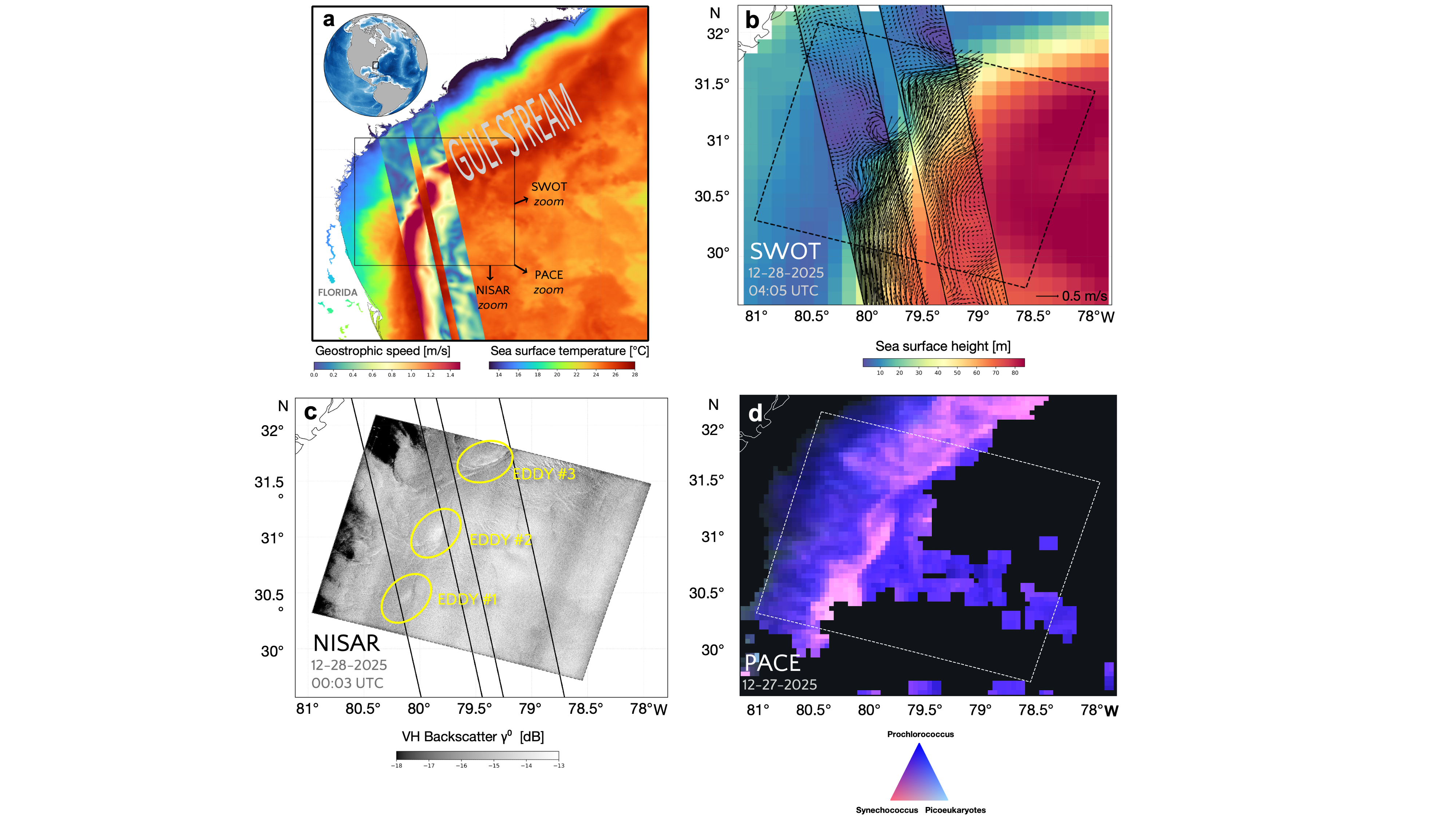
| Panel | Content |
|---|---|
| a | MUR L4 SST background + SWOT L3 geostrophic speed swath + NISAR footprint box |
| b | MIOST v3 ADT background + SWOT ADT swath + swath-edge bars + geostrophic velocity quiver |
| c | NISAR L2 GCOV VH (VHVH) gamma-naught backscatter, grayscale |
| d | PACE OCI MOANA picophytoplankton ternary composite |
Figure 2 — SWOT L2 ADT x VIIRS SST & chlorophyll triptych (1x3)
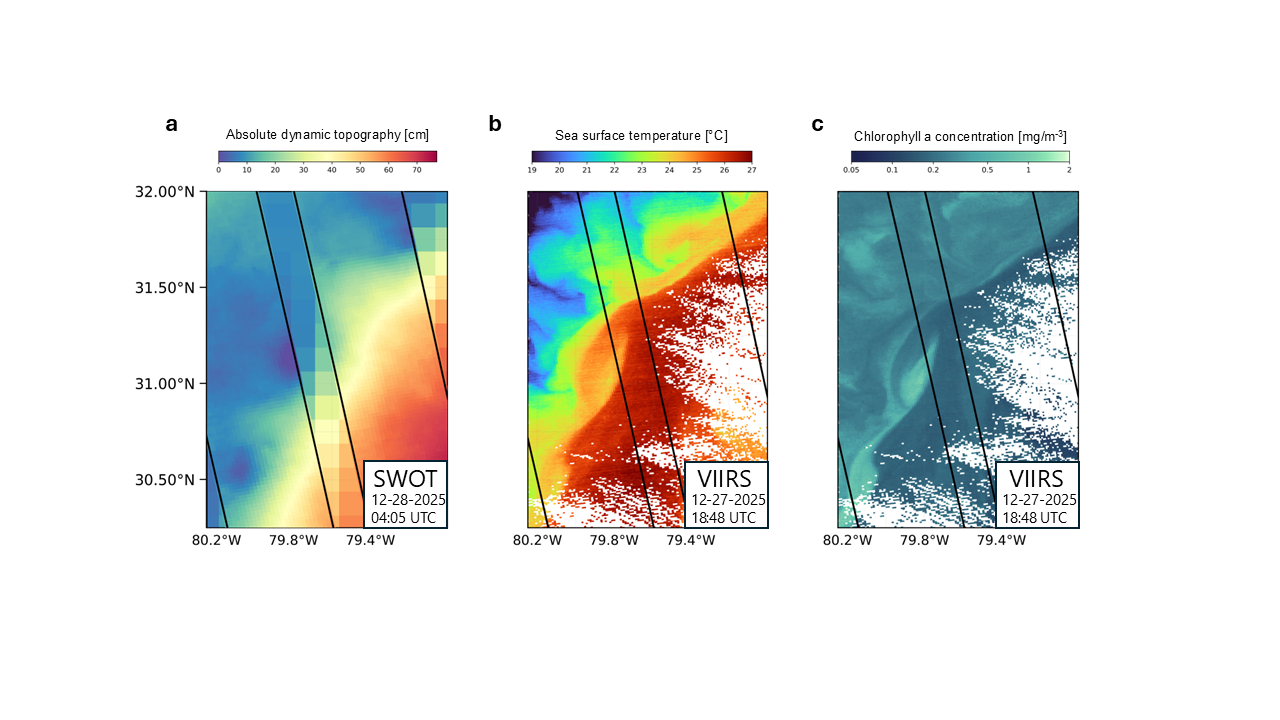
| Panel | Content |
|---|---|
| a | SWOT JPL L2 ADT swath over MIOST v3 ADT (also rendered without the background) |
| b | VIIRS SST, masked to the chlorophyll panel’s valid pixels |
| c | VIIRS log10(chlorophyll a), colorbar ticked in mg m-3 |
SWOT ADT is formed from the L2 LR SSH Expert product as (ssha_karin + height_cor_xover) + mean_dynamic_topography
Setup
Install the Python dependencies (numpy, xarray, netCDF4, h5py, scipy, matplotlib, cartopy, rasterio). cartopy and rasterio need system libraries (GEOS / PROJ / GDAL) and install most reliably with conda:
conda env create -f environment.yml
conda activate swot-dia
Or with pip (see the note in requirements.txt if cartopy/rasterio fail to build):
pip install -r requirements.txtData
The satellite data is not included — you download it yourself (free NASA Earthdata and AVISO accounts). See DATA.md for exactly what to download and where to get it, then place the files in the shared data root (~/Data/<source>/..., outside the repo):
- SWOT L3 LR SSH Expert (AVISO/DUACS) and SWOT L2 LR SSH Expert (JPL PO.DAAC)
- NISAR L2 GCOV (ASF DAAC)
- MUR L4 SST (JPL PO.DAAC GHRSST)
- MIOST v3 gridded ADT (AVISO)
- PACE OCI L4 MOANA picophytoplankton (NASA OB.DAAC)
- SNPP VIIRS L2 SST and Ocean Color (NASA OB.DAAC)
- ETOPO 2022 30 arc-second surface elevation (NOAA NCEI) — streamed at run time, no download
Files are located by glob pattern within each dataset’s shared-root sub-folder (searched recursively), so exact filenames are flexible. The shared root defaults to ~/Data; override it with the DATA_ROOT environment variable (legacy SWOT_DIA_DATA_DIR still works).
Quickstart
cd "Data in Action Figure 1"
python Figure1.py            # full composite + all pieces -> ./pieces/
python Figure1_panelC.py     # or just one panel
Each script writes its output PNGs into that figure’s pieces/ folder. If a data file is missing, the script stops with a clear message naming the expected file and pointing to DATA.md. Run the .ipynb equivalents instead if you prefer notebooks.
Layout
Each figure directory contains:
FigureN.py / .ipynb            composite(s) + every piece
FigureN_panelX.py / .ipynb     one panel on its own, with its pieces
figureN_common.py              shared config, loaders, draw primitives, piece renderer
FigureN_composite*.png         layout reference
pieces/                        the exported figure elements
The .py and .ipynb versions of each script are equivalent (jupytext percent format); run either.