From the PO.DAAC Cookbook, to access the GitHub version of the notebook, follow this link.

Exploring gauges and river discharge in the SWORD of Science (SoS) dataset

Author: Nikki Tebaldi, NASA JPL PO.DAAC

Summary

Looking at discharge in the SoS

It can be helpful to plot the flow law parameter estimation (FLPE) algorithm discharge alongside the integrator (MOI) discharge produced for that algorithm PLUS overlapping in situ gauge data. Note that not all rivers have gauge data associated with them. In this notebook we will look at the steps to plot SoS discharge values produced from running the Confluence workflow alongside in situ gauge data gathered and stored in the priors.

Granule structure (background)

The SWORD of Science (SoS) is a community-driven dataset produced for and from the execution of the Confluence workflow in the cloud which enables quick data access and compute on SWOT data. Data granules contain two files, priors and results. The priors file contains prior information, such as in-situ gage data and model output that is used to generate the discharge products. The results file contains the resulting river discharge data products.

The cloud-based workflow (“Confluence”) that produces the SoS will produce discharge parameter estimates which the SWOT mission will use to produce discharge. This discharge will be stored in the SWOT shapefiles as the official SWOT discharge. However, the Confluence workflow produces discharge time series alongside the discharge parameter estimates in order to preview what will eventually stored in the SWOT shapefiles. Users can reference the SoS for the latest discharge time series recognizing that the official SWOT discharge data product lives in the SWOT shapefiles.

The SoS is organized by continent following SWOT River Database (SWORD) structure and naming conventions. It is indexed on the same reach and node identifier dimensions found in SWORD. Time series data is stored by cycle and pass on an observation dimension.

More information is available in the SWOT-Confluence Github repository: * Documentation for priors * Documentation for results

Results are organized into groups corresponding to modules in the SWOT-Confluence processing software. Modules are described in the Confluence Module Documentation.

You can explore the SoS further in this notebook: https://podaac.github.io/tutorials/notebooks/datasets/SWOT_L4_DAWG_SOS_DISCHARGE.html

Locate data for a river that has gauges

We will select the Ohio River as we know it has gauge data associated with it from the USGS but feel free to modify the constants below for your river of choice!

Table of Gauge Agencies by Continent

The following list the continent with associated gauge agency and group name of the gauge agency as it is stored in the SoS.

Continent	Group Name	Gauge Agency
Africa	GRDC	Global Runoff Data Centre
Asia	GRDC	Global Runoff Data Centre
Asia	MLIT	Ministry of Land, Infrastructure, Transport, Tourism
Europe	GRDC	Global Runoff Data Centre
Europe	DEFRA	Department of Environment Food & Rural Affairs
Europe	EAU	Hub’Eau France
North America	GRDC	Global Runoff Data Centre
North America	USGS	United State Geological Survey
North America	WSC	Water Survey Canada
Oceania	GRDC	Global Runoff Data Centre
Oceania	ABOM	Australian Government Bureau of Meteorology
South America	GRDC	Global Runoff Data Centre
South America	DGA	Direccion General de Aguas
South America	Hidroweb	Hidroweb

Requirements

1. Compute environment

This tutorial can be run in the following environments: - Local compute environment e.g. laptop, server: this tutorial can be run on your local machine

2. Earthdata Login

An Earthdata Login account is required to access data, as well as discover restricted data, from the NASA Earthdata system. Thus, to access NASA data, you need Earthdata Login. Please visit https://urs.earthdata.nasa.gov to register and manage your Earthdata Login account. This account is free to create and only takes a moment to set up.

Learning Objectives

• To locate in situ gauge data stored in the SoS.
• To locate overlap between in situ observations and times where discharge values were produced.
• Plot gauge data alongside river discharge.

---

Import Packages

import datetime
import pathlib

import cartopy.crs as ccrs
import cartopy.feature as cfeature
from cartopy.mpl.gridliner import LONGITUDE_FORMATTER, LATITUDE_FORMATTER
import earthaccess
import matplotlib.pyplot as plt
import netCDF4 as nc
import numpy as np
import pandas as pd

Authenticate

Authenticate your Earthdata Login (EDL) information using the earthaccess python package as follows:

earthaccess.login() # Login with your EDL credentials if asked

<earthaccess.auth.Auth at 0x31276f1d0>

Search and Access SoS data

Locate the SoS data of interest and then download for access.

# Search and locate granules
granule_info = earthaccess.search_data(
    short_name="SWOT_L4_DAWG_SOS_DISCHARGE",
    temporal=("2023-04-07", "2023-04-26"),
)
granule_info

Granules found: 3

[Collection: {'Version': '1', 'ShortName': 'SWOT_L4_DAWG_SOS_DISCHARGE'}
 Spatial coverage: {'HorizontalSpatialDomain': {'Geometry': {'BoundingRectangles': [{'WestBoundingCoordinate': -21.794, 'SouthBoundingCoordinate': 25.382, 'EastBoundingCoordinate': 25.382, 'NorthBoundingCoordinate': 81.115}]}}}
 Temporal coverage: {'RangeDateTime': {'EndingDateTime': '2023-04-25T20:01:59.000Z', 'BeginningDateTime': '2023-04-07T22:49:35.000Z'}}
 Size(MB): 983.0999364852905
 Data: ['https://archive.podaac.earthdata.nasa.gov/podaac-ops-cumulus-protected/SWOT_L4_DAWG_SOS_DISCHARGE/eu_sword_v15_SOS_unconstrained_0001_20240228T205029_results.nc', 'https://archive.podaac.earthdata.nasa.gov/podaac-ops-cumulus-protected/SWOT_L4_DAWG_SOS_DISCHARGE/eu_sword_v15_SOS_unconstrained_0001_20240228T205029_priors.nc'],
 Collection: {'Version': '1', 'ShortName': 'SWOT_L4_DAWG_SOS_DISCHARGE'}
 Spatial coverage: {'HorizontalSpatialDomain': {'Geometry': {'BoundingRectangles': [{'WestBoundingCoordinate': -81.139, 'SouthBoundingCoordinate': -52, 'EastBoundingCoordinate': -52, 'NorthBoundingCoordinate': 11.097}]}}}
 Temporal coverage: {'RangeDateTime': {'EndingDateTime': '2023-04-26T12:04:55.000Z', 'BeginningDateTime': '2023-04-08T01:51:07.000Z'}}
 Size(MB): 1700.4334163665771
 Data: ['https://archive.podaac.earthdata.nasa.gov/podaac-ops-cumulus-protected/SWOT_L4_DAWG_SOS_DISCHARGE/sa_sword_v15_SOS_unconstrained_0001_20240228T205034_results.nc', 'https://archive.podaac.earthdata.nasa.gov/podaac-ops-cumulus-protected/SWOT_L4_DAWG_SOS_DISCHARGE/sa_sword_v15_SOS_unconstrained_0001_20240228T205034_priors.nc'],
 Collection: {'Version': '1', 'ShortName': 'SWOT_L4_DAWG_SOS_DISCHARGE'}
 Spatial coverage: {'HorizontalSpatialDomain': {'Geometry': {'BoundingRectangles': [{'WestBoundingCoordinate': -166.397, 'SouthBoundingCoordinate': 8.09, 'EastBoundingCoordinate': 8.09, 'NorthBoundingCoordinate': 82.311}]}}}
 Temporal coverage: {'RangeDateTime': {'EndingDateTime': '2023-04-26T13:28:35.000Z', 'BeginningDateTime': '2023-04-08T05:36:12.000Z'}}
 Size(MB): 1613.2776679992676
 Data: ['https://archive.podaac.earthdata.nasa.gov/podaac-ops-cumulus-protected/SWOT_L4_DAWG_SOS_DISCHARGE/na_sword_v15_SOS_unconstrained_0001_20240228T205032_results.nc', 'https://archive.podaac.earthdata.nasa.gov/podaac-ops-cumulus-protected/SWOT_L4_DAWG_SOS_DISCHARGE/na_sword_v15_SOS_unconstrained_0001_20240228T205032_priors.nc']]

# Enter a directory path to store downloaded data in
downloads_dir = pathlib.Path("data_downloads")
downloads_dir.mkdir(parents=True, exist_ok=True)

# Select a priors and results pair to explore
download_links = [[link for link in earthaccess.results.DataGranule.data_links(granule)] for granule in granule_info]
print("Select a priors and results file to explore:")
for downloads in download_links: 
    for download in downloads:
        if "priors" in download: print(download)

Select a priors and results file to explore:
https://archive.podaac.earthdata.nasa.gov/podaac-ops-cumulus-protected/SWOT_L4_DAWG_SOS_DISCHARGE/eu_sword_v15_SOS_unconstrained_0001_20240228T205029_priors.nc
https://archive.podaac.earthdata.nasa.gov/podaac-ops-cumulus-protected/SWOT_L4_DAWG_SOS_DISCHARGE/sa_sword_v15_SOS_unconstrained_0001_20240228T205034_priors.nc
https://archive.podaac.earthdata.nasa.gov/podaac-ops-cumulus-protected/SWOT_L4_DAWG_SOS_DISCHARGE/na_sword_v15_SOS_unconstrained_0001_20240228T205032_priors.nc

# Select Europe ("eu") priors file to work with
priors_link = "https://archive.podaac.earthdata.nasa.gov/podaac-ops-cumulus-protected/SWOT_L4_DAWG_SOS_DISCHARGE/eu_sword_v15_SOS_unconstrained_0001_20240228T205029_priors.nc"

# Select results
results_link = priors_link.replace("priors", "results")

earthaccess.download(priors_link, downloads_dir)
earthaccess.download(results_link, downloads_dir)

File eu_sword_v15_SOS_unconstrained_0001_20240228T205029_priors.nc already downloaded

File eu_sword_v15_SOS_unconstrained_0001_20240228T205029_results.nc already downloaded

['data_downloads/eu_sword_v15_SOS_unconstrained_0001_20240228T205029_results.nc']

# Open downloaded files to access SoS granule data
priors_download = priors_link.split('/')[-1]
results_download = results_link.split('/')[-1]

priors = nc.Dataset(downloads_dir.joinpath(priors_download), format="NETCDF4")
results = nc.Dataset(downloads_dir.joinpath(results_download), format="NETCDF4")

Locate gauge and rive discharge data.

We can now locate gauge and river discharge data from the SoS using either the data read directly from S3 or downloaded to your local computer.

# Constants

# Select a river
RIVER_NAME = "Rhine"

# Select a discharge algorithm (hivdi, neobam, metroman, momma, sad, sic4dvar)
DISCHARGE_ALGORITHM = "hivdi"
DISCHARGE_VARIABLE = "Q"

# Select a gauge agency
GAUGE_AGENCY = "EAU"

Locate overlapping identifiers

Locate overlapping identifiers for reach and gauge data.

# Locate overlapping reach identifier
river_names = results['reaches']['river_name'][:]
river_indexes = np.where(river_names  == RIVER_NAME)

river_reach = results["reaches"]["reach_id"][river_indexes]
print(f"{RIVER_NAME} reach identifiers:")
print(river_reach)

gauge_reach = priors[GAUGE_AGENCY][f"{GAUGE_AGENCY}_reach_id"][:]
print("Gauge reach identifiers:")
print(gauge_reach)

reach_overlap = np.intersect1d(gauge_reach, river_reach)
print("Overlapping reaches:")
print(reach_overlap)

# Select the first reach
reach_id = reach_overlap[0]
print(f"Reach id selected: {reach_id}")

Rhine reach identifiers:
[23261000181 23261000191 23261000201 23261000211 23261000221 23261000231
 23261000241 23261000274 23261000371 23261000381 23261000391 23261000401
 23261000411 23261000421 23261000431 23261000441 23261000451 23261000461
 23261000471 23261000481 23261000491 23261000501 23261000511 23261000521
 23261000561 23261000571 23261000581 23261000621 23261000631 23261000641
 23262000011 23263000011 23263000021 23263000031 23263000061 23263000071
 23263000081 23263000091 23263000141 23263000151 23263000161 23263000211
 23263000221 23263000231 23263000241 23263000251 23263000271 23263000281
 23265000021 23265000031 23265000041 23265000051 23265000061 23267000011
 23267000021 23267000031 23267000041 23267000051 23267000061 23267000071
 23267000081 23267000094 23267000101 23267000111 23267000121 23267000131
 23267000141 23267000154 23267000171 23267000181 23267000194 23267000214
 23267000224 23267000231 23267000244 23267000304 23267000361 23267000371
 23267000384 23267000391 23267000401 23267000414 23267000494 23267000501
 23267000511 23267000524 23267000531 23267000541 23267000551 23267000561
 23267000571 23267000584 23267000591 23267000604 23267000611 23267000624
 23267000631 23267000644 23267000651 23267000664 23267000671 23267000684
 23267000704 23267000711 23267000724 23267000731 23267000744 23269000024
 23269000031 23269000051 23269000101 23269000114 23269000121 23269000134
 23269000141 23269000214 23269000221 23269000234 23269000241 23269000254
 23269000261 23269000271 23269000283 23269000293 23269000311 23269000323
 23269000333 23269000343 23269000353 23269000371 23269000381 23269000714
 23269000721 23269000734 23269000741 23269000754 23269000761 23269000774
 23269000781 23269000794 23269000801 23269000814 23269000824 23269000831
 23269000841 23269000941]
Gauge reach identifiers:
[23267000501 23267000121 23267000121 23267000081 23267000081 23267000071
 23262000901 23262000801 23262000801 23262000731 23262001444 23262001104
 23262001061 23262001354 23262000551 23262000531 23262000511 23262000491
 23262001394 23250801191 23250200011 23250600821 23250600484 23250600471
 23250600441 23250600631 23250200441 23240600314 23240602811 23240600201
 23240600261 23240600091 23240700491 23240700321 23240700181 23240700081
 23240700021 23240500101 23240500101 23240600431 23240603204 23240400101
 23240602381 23240602651 23240100201 23240900074 23240900151 23240700541
 23240700464 23240400601 23240400491 23240400414 23240400291 23230500654
 23230500401 23230500301 23230500081 23230400101 23230400101 23230200764
 23230200744 23230200354 23230200331 23230200986 23230200434 23230200381
 23230200965 23229000554 23229000211 23229000131 23229000521 23229000101
 23229000431 23229000024 23228000341 23228000231 23228000151 23228000111
 23228000091 23227000261 23227000231 23227000181 23227000181 23227000111
 23227000101 23227000041 23227000011 23226000564 23226000461 23226000351
 23226000321 23226000311 23226000031 23225000031 23224001551 23224001174
 23224000821 23224000531 23224000391 23224000331 23224000121 23224000704
 23224000661 23224000601 23224000601 23224000241 23224000861 23224000191
 23224000021 23223000041 23222000351 23222000661 23222001144 23222000801
 23222000011 23221000224 23219000444 23219000071 23214400931 23214400791
 23214401114 23214400501 23214400111 23214400201 23214400151 23214400041
 23214400013 23214900374 23214900361 23214900261 23214900224 23214900014
 23214700141 23214700051 23214700011 23214600374 23214600144 23214300031
 23214201131 23214200904 23214200691 23214200564 23214200531 23214200091
 23214200011 23214100051 23214100031 23214100155 23216000611 23216000584
 23216000561 23216000511 23216000501 23216000441 23216000421 23216000401
 23216001061 23216001001 23216000721 23212001134 23212001081 23212001014
 23212000701 23212000674 23212001366 23212000071 23212000051 23212000834
 23212000364 23212000181 23212001345 23218000304 23218000381 23218000141
 23218000121 23218000101 21602801794 21602800144 21602902191 21602902121
 21602901924 21602901501 21602900954 21602700241 21602700121 21602700171
 21602700011 21602602314 21602602351 21602601944 21602601393 21602601373
 21602601363 21602600311 21602601251 21602601231 21602601231 21602601821
 21602602381 21602600631 21602600011 21602300471 21602300441 21602300241
 21602300774 21602300861 21602300664 21602300221 21602300131 21602300131
 21602300351 21602100401 21602100264 21602100181 21602100144 21602100535
 21602100535 21602400711 21602400761 21602400751 21602400744 21602401061
 21602400221 21602400201 21602200354 21602200681 21602200204 21602200084
 21603400261 21603400161 21603400141 21603400091 21603400064 21603400051
 21603200231 21603200261 21603200191 21603300181 21603300154 21603300061
 21601000171 21601000091 21601000013]
Overlapping reaches:
[23267000071 23267000081 23267000121 23267000501]
Reach id selected: 23267000071

Locate gauge discharge and in situ observation time

Locate discharge and save the in situ observation time for the reach of interest.

# Get reach index for gauge data
reach_gauge_index = np.where(gauge_reach == reach_id)

# Get discharge and filter out missing values
missing = priors[GAUGE_AGENCY][f"{GAUGE_AGENCY}_q"]._FillValue
gauge_discharge = priors[GAUGE_AGENCY][f"{GAUGE_AGENCY}_q"][reach_gauge_index].filled()[0]
nonmissing_indexes_g = np.where(gauge_discharge != missing)
gauge_discharge = gauge_discharge[nonmissing_indexes_g]
print(f"Number of gauge discharge values: {len(gauge_discharge)}.")

# Get time and filter out missing values
gauge_time = priors[GAUGE_AGENCY][f"{GAUGE_AGENCY}_qt"][reach_gauge_index].filled().astype(int)[0]
gauge_time = gauge_time[nonmissing_indexes_g]
print(f"Number of gauge time values: {len(gauge_time)}.")

# Convert time from ordinal value
gauge_time = [ datetime.datetime.fromordinal(gt).strftime("%Y%m%d") for gt in gauge_time ]

Number of gauge discharge values: 3722.
Number of gauge time values: 3722.

Locate algorithm discharge

Locate the algorithm discharge for a corresponding reach identifier that has gauge data. We will use HiVDI for this demonstration.

# Locate the reach identifier and associated discharge time series
reach_q_index = np.where(results['reaches']['reach_id'][:] == reach_id)
print("Reach Index: ", reach_q_index)
discharge_q = results[DISCHARGE_ALGORITHM][DISCHARGE_VARIABLE][reach_q_index][0]

# Filter out missing values
missing = results[DISCHARGE_ALGORITHM][DISCHARGE_VARIABLE].missing_value
nonmissing_indexes = np.where(discharge_q != missing)
discharge_q = discharge_q[nonmissing_indexes]
print(f"Number of {DISCHARGE_ALGORITHM.upper()} discharge values: {len(discharge_q)}.")
print(discharge_q)

# Retrieve SWOT observation times and filter out missing values
time = results['reaches']['time'][reach_q_index][0]
time = time[nonmissing_indexes]

# Convert to discharge time to same format as gauge agency time
swot_ts = datetime.datetime(2000,1,1,0,0,0)   # SWOT timestamp delta
discharge_time = [ (swot_ts + datetime.timedelta(seconds=st)).strftime("%Y%m%d") for st in time ]
print(f"Number of {DISCHARGE_ALGORITHM.upper()} time values: {len(time)}.")
print(discharge_time)

Reach Index:  (array([13158]),)
Number of HIVDI discharge values: 7.
[1213.67194541 1138.18496353 1115.0978839  1069.45943177 1082.94584138
 1198.94024353 1108.93895269]
Number of HIVDI time values: 7.
['20230418', '20230419', '20230420', '20230422', '20230423', '20230424', '20230425']

Locate integrator (MOI) discharge

Locate the integrator discharge produced for the algorithm for the reach of interest that has gauge data. As mentioned, we will use HiVDI for this demonstration.

# Locate MOI discharge results for discharge algorithm making sure to filter out missing values
moi_q = results["moi"][DISCHARGE_ALGORITHM]["q"][reach_q_index][0]
moi_q = moi_q[nonmissing_indexes]

# Set missing MOI to NaN
missing_moi = results["moi"][DISCHARGE_ALGORITHM]["q"].missing_value
moi_q[moi_q == missing_moi] = np.nan
print(f"Number of integrator {DISCHARGE_ALGORITHM.upper()} discharge values: {len(moi_q)}.")
print(moi_q)

Number of integrator HIVDI discharge values: 7.
[334.24668321 297.51701118 290.62386718 259.68934869 261.49240103
 307.47902449 288.01774716]

Locate overlapping observations

We will need to locate the discharge time series (FLPE and MOI) for the Rhine reach of interest and then determine if there are overlapping in situ observations with SWOT observations.

# Find overlapping time between in situ and SWOT observations
obs_overlap = list(set(discharge_time).intersection(set(gauge_time)))
obs_overlap.sort()
print("Days of observation overlap:")
print(obs_overlap)

# Get indexes of overlap for gauge, algorithm and integrator
gauge_overlap_index = np.where(np.in1d(gauge_time, obs_overlap))[0]
discharge_overlap_index = np.where(np.in1d(discharge_time, obs_overlap))[0]

# Retrieve time and discharge values for indexes
gauge_time = np.array(gauge_time)[gauge_overlap_index]
gauge_discharge = np.array(gauge_discharge)[gauge_overlap_index]
# print("Gauge time:\n", gauge_time)
print("Gauge discharge:\n", gauge_discharge)

discharge_time = np.array(discharge_time)[discharge_overlap_index]
discharge_algo = np.array(discharge_q)[discharge_overlap_index]
# print(f"{DISCHARGE_ALGORITHM} time:\n", discharge_time)
print(f"{DISCHARGE_ALGORITHM} discharge:\n", discharge_algo)

moi_q = np.array(moi_q)[discharge_overlap_index]
print(f"MOI discharge for {DISCHARGE_ALGORITHM}:\n", moi_q)

Days of observation overlap:
['20230418', '20230419', '20230420', '20230422', '20230423', '20230424', '20230425']
Gauge discharge:
 [1334.333 1208.255 1148.526 1115.296 1077.891 1080.885 1153.646]
hivdi discharge:
 [1213.67194541 1138.18496353 1115.0978839  1069.45943177 1082.94584138
 1198.94024353 1108.93895269]
MOI discharge for hivdi:
 [334.24668321 297.51701118 290.62386718 259.68934869 261.49240103
 307.47902449 288.01774716]

Plotting results for comparison

Let’s plot all discharge time series to better visualize the differences and compare the FLPE, MOI, and gauge discharge values.

# Plot discharge alongside MOI discharge and gauge discharge

# Discharge algorithm Q
plt.scatter(discharge_time, discharge_algo)
plt.plot(discharge_time, discharge_algo, label=f"{DISCHARGE_ALGORITHM.upper()}")

# MOI Q
plt.scatter(discharge_time, moi_q)
plt.plot(discharge_time, moi_q, label="MOI")

# Gauge Q
plt.scatter(gauge_time, gauge_discharge)
plt.plot(gauge_time, gauge_discharge, label="Gauge")

plt.suptitle(f"Discharge Timeseries from {DISCHARGE_ALGORITHM} for the {RIVER_NAME} reach identifier: {reach_id}.")
plt.legend()
plt.tight_layout()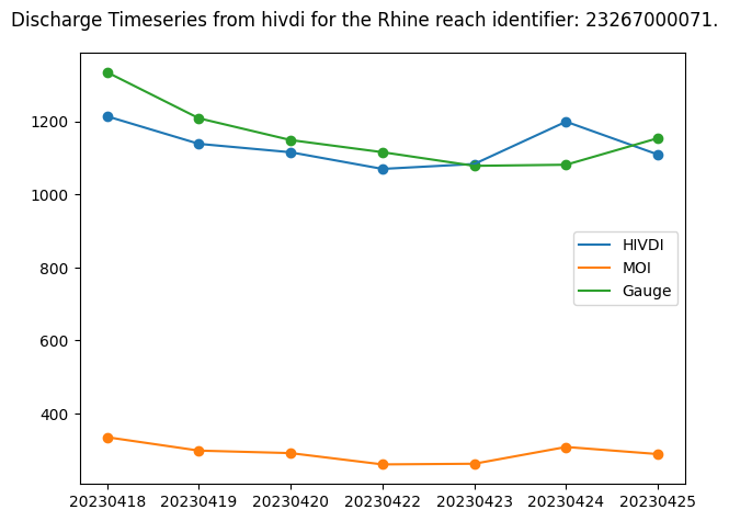

---

Disclaimer: Reference herein to any specific commercial product, process, or service by trade name, trademark, manufacturer, or otherwise, does not constitute or imply its endorsement by the United States Government or the Jet Propulsion Laboratory, California Institute of Technology.