Zarr Example

imported on: 2024-10-30

This notebook is from NASA’s Zarr EOSDIS store notebook

The original source for this document is https://github.com/nasa/zarr-eosdis-store/blob/main/presentation/example.ipynb

zarr-eosdis-store example

Install dependencies

import sys

# zarr and zarr-eosdis-store, the main libraries being demoed
!{sys.executable} -m pip install zarr zarr-eosdis-store

# Notebook-specific libraries
!{sys.executable} -m pip install matplotlib

Important: To run this, you must first create an Earthdata Login account (https://urs.earthdata.nasa.gov) and place your credentials in ~/.netrc e.g.:

   machine urs.earthdata.nasa.gov login YOUR_USER password YOUR_PASSWORD

Never share or commit your password / .netrc file!

Basic usage. After these lines, we work with ds as though it were a normal Zarr dataset

import zarr
from eosdis_store import EosdisStore

url = 'https://archive.podaac.earthdata.nasa.gov/podaac-ops-cumulus-protected/MUR-JPL-L4-GLOB-v4.1/20210715090000-JPL-L4_GHRSST-SSTfnd-MUR-GLOB-v02.0-fv04.1.nc'

ds = zarr.open(EosdisStore(url))

View the file’s variable structure

print(ds.tree())

/
 ├── analysed_sst (1, 17999, 36000) int16
 ├── analysis_error (1, 17999, 36000) int16
 ├── dt_1km_data (1, 17999, 36000) int16
 ├── lat (17999,) float32
 ├── lon (36000,) float32
 ├── mask (1, 17999, 36000) int16
 ├── sea_ice_fraction (1, 17999, 36000) int16
 ├── sst_anomaly (1, 17999, 36000) int16
 └── time (1,) int32

Fetch the latitude and longitude arrays and determine start and end indices for our area of interest. In this case, we’re looking at the Great Lakes, which have a nice, recognizeable shape. Latitudes 41 to 49, longitudes -93 to 76.

lats = ds['lat'][:]
lons = ds['lon'][:]
lat_range = slice(lats.searchsorted(41), lats.searchsorted(49))
lon_range = slice(lons.searchsorted(-93), lons.searchsorted(-76))

Get the analysed sea surface temperature variable over our area of interest and apply scale factor and offset from the file metadata. In a future release, scale factor and add offset will be automatically applied.

var = ds['analysed_sst']
analysed_sst = var[0, lat_range, lon_range] * var.attrs['scale_factor'] + var.attrs['add_offset']

Draw a pretty picture

from matplotlib import pyplot as plt

plt.rcParams["figure.figsize"] = [16, 8]
plt.imshow(analysed_sst[::-1, :])
None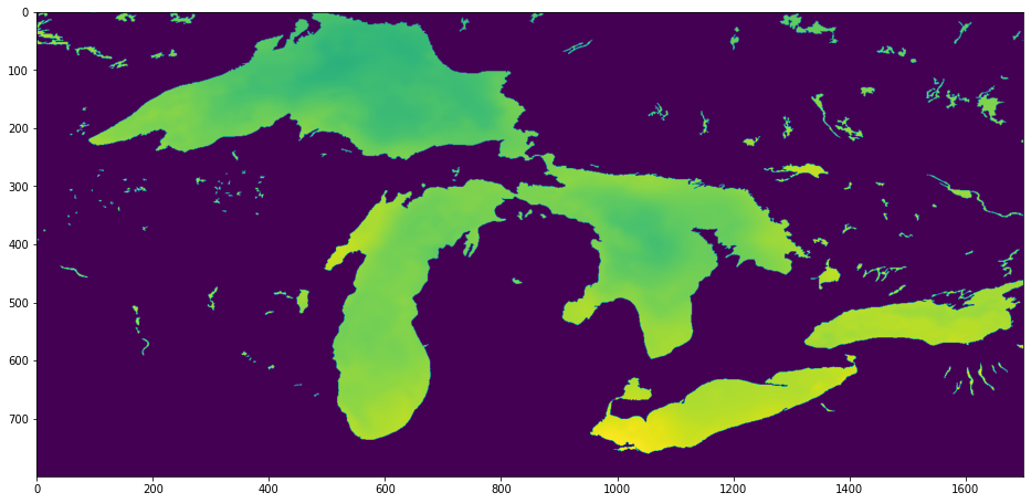

In a dozen lines of code and a few seconds, we have managed to fetch and visualize the 3.2 megabyte we needed from a 732 megabyte file using the original archive URL and no processing services