Explore Gulf of Tehuantepec extreme wind events and ocean response

Import Packages

Note using Zarr Version 2

Successfully tested with the following critical component versions: kerchunk==0.2.7, virtualizarr–1.3.2, xarray==2025.4.0 zarr==2.18.7

#pip install earthaccess==0.13.0 zarr==2.18.7 fastparquet==2024.5.0 xarray==2025.4.0 fsspec==2024.10.0 "dask[complete]"==2024.5.2 h5netcdf==1.3.0 ujson==5.10.0 matplotlib==3.9.2  kerchunk==0.2.7 virtualizarr==1.3.2  cftime cartopy

pip list | grep -E "zarr|xarray|virtualizarr|kerchunk"

kerchunk                  0.2.7
virtualizarr              1.3.2
xarray                    2025.4.0
zarr                      2.18.7
Note: you may need to restart the kernel to use updated packages.

# Built-in packages
import os
import sys

# Filesystem management 
import fsspec
import earthaccess

# Data handling
import xarray as xr
import numpy as np

# Parallel computing 
import multiprocessing
from dask import delayed
import dask.array as da
from dask.distributed import Client

# Other
import matplotlib.pyplot as plt
import cartopy.crs as ccrs
import cartopy.feature as cfeature

Other Setup

xr.set_options( # display options for xarray objects
    display_expand_attrs=False,
    display_expand_coords=True,
    display_expand_data=True,
)

<xarray.core.options.set_options at 0x7fcc21080b90>

1. Obtaining credentials and generating a VDS mapper

The first step is to find the S3 or https endpoints to the files. Handling access credentials to Earthdata and then finding the endpoints can be done a number of ways (e.g. using the requests, s3fs packages) but we use the earthaccess package for its ease of use.

# Get Earthdata creds
earthaccess.login()

Enter your Earthdata Login username:  edward.m.armstrong
Enter your Earthdata password:  ········

<earthaccess.auth.Auth at 0x7fcbfff54920>

In the next step we define a generic VDS wrapper and that can be wrapped into a function (no modification needed). The mapper will contain all the required access credentials and can be passed directly to xarray. In the future this step will likely be built into to earthaccess but for now we must define it in the notebook. The only inputs to the function are:

1. The link to the VDS reference file.
2. Whether or not you are accessing the data in the cloud in the same region as the data. For most beginning users this argument will be set to False.

def get_vds_mapper(vds_link, in_cloud_region=False):
    """
    Produces a virtudal dataset mapper that can be passed to xarray. 
    
    * vds_link: str, link to the mapper
    * in_cloud_region: bool, True if in cloud in the same region as the data, 
        False otherwise.
    """

    if in_cloud_region:
        fs_data = earthaccess.get_s3_filesystem(daac="PODAAC")
        remote_protocol = "s3"
    else:
        fs_data = earthaccess.get_fsspec_https_session()
        remote_protocol = "https"
    
    storage_opts = {"fo": vds_link, "remote_protocol": remote_protocol, "remote_options": fs_data.storage_options}
    fs_ref = fsspec.filesystem('reference', **storage_opts)
    return fs_ref.get_mapper('')

2. Open reference files

OSTIA Daily Sea Surface Temperature (OSTIA-UKMO-L4-GLOB-REP-v2.0)

%%time
# Open the OSTIA Reprocessed SST reference file (OSTIA-UKMO-L4-GLOB-REP-v2.0)
vds_link = 'https://archive.podaac.earthdata.nasa.gov/podaac-ops-cumulus-public/virtual_collections/OSTIA-UKMO-L4-GLOB-REP-v2.0/OSTIA-UKMO-L4-GLOB-REP-v2.0_virtual_https.json'
vds_mapper = get_vds_mapper(vds_link, in_cloud_region=False)

CPU times: user 549 ms, sys: 191 ms, total: 741 ms
Wall time: 3.01 s

%%time

## No modification needed. Read as xarray dataset.
sst_ds = xr.open_dataset(
    vds_mapper, engine="zarr", chunks={},
    backend_kwargs={"consolidated": False}
)
sst_ds

CPU times: user 588 ms, sys: 43 ms, total: 631 ms
Wall time: 642 ms

<xarray.Dataset> Size: 11TB
Dimensions:           (time: 15340, lat: 3600, lon: 7200)
Coordinates:
  * lat               (lat) float32 14kB -89.97 -89.93 -89.88 ... 89.93 89.97
  * lon               (lon) float32 29kB -180.0 -179.9 -179.9 ... 179.9 180.0
  * time              (time) datetime64[ns] 123kB 1982-01-01T12:00:00 ... 202...
Data variables:
    analysed_sst      (time, lat, lon) float64 3TB dask.array<chunksize=(1, 1200, 2400), meta=np.ndarray>
    analysis_error    (time, lat, lon) float64 3TB dask.array<chunksize=(1, 1200, 2400), meta=np.ndarray>
    mask              (time, lat, lon) float32 2TB dask.array<chunksize=(1, 1800, 3600), meta=np.ndarray>
    sea_ice_fraction  (time, lat, lon) float64 3TB dask.array<chunksize=(1, 1800, 3600), meta=np.ndarray>
Attributes: (39)

CCMP 6 Hourly Ocean Winds (CCMP_WINDS_10M6HR_L4_V3.1)

%%time

# Open the CCMP Winds reference file (CCMP_WINDS_10M6HR_L4_V3.1)
vds_link = 'https://archive.podaac.earthdata.nasa.gov/podaac-ops-cumulus-public/virtual_collections/CCMP_WINDS_10M6HR_L4_V3.1/CCMP_WINDS_10M6HR_L4_V3.1_virtual_https.json'
vds_mapper = get_vds_mapper(vds_link, in_cloud_region=False)

wind_ds = xr.open_dataset(
    vds_mapper, engine="zarr", chunks={},
    backend_kwargs={"consolidated": False}
)
wind_ds

CPU times: user 599 ms, sys: 52.3 ms, total: 651 ms
Wall time: 1.85 s

<xarray.Dataset> Size: 781GB
Dimensions:    (latitude: 720, longitude: 1440, time: 47056)
Coordinates:
  * latitude   (latitude) float32 3kB -89.88 -89.62 -89.38 ... 89.38 89.62 89.88
  * longitude  (longitude) float32 6kB 0.125 0.375 0.625 ... 359.4 359.6 359.9
  * time       (time) datetime64[ns] 376kB 1993-01-02 ... 2025-03-31T18:00:00
Data variables:
    nobs       (time, latitude, longitude) float32 195GB dask.array<chunksize=(1, 720, 1440), meta=np.ndarray>
    uwnd       (time, latitude, longitude) float32 195GB dask.array<chunksize=(1, 720, 1440), meta=np.ndarray>
    vwnd       (time, latitude, longitude) float32 195GB dask.array<chunksize=(1, 720, 1440), meta=np.ndarray>
    ws         (time, latitude, longitude) float32 195GB dask.array<chunksize=(1, 720, 1440), meta=np.ndarray>
Attributes: (44)

# Determine and append the wind direction to the wind_ds dataset

# Calculate wind direction in degrees using arctan2(-u, -v)
wind_dir = np.arctan2(-wind_ds.uwnd, -wind_ds.vwnd)  # radians
wind_dir = np.degrees(wind_dir)  # convert to degrees
wind_dir = (wind_dir + 360) % 360  # ensure values are between 0 and 360

# Assign to dataset
wind_ds['wind_direction'] = wind_dir
wind_ds['wind_direction'].attrs.update({
    'units': 'degrees',
    'standard_name': 'wind_from_direction',
    'long_name': 'Wind Direction (meteorological)'
})
wind_ds

<xarray.Dataset> Size: 976GB
Dimensions:         (latitude: 720, longitude: 1440, time: 47056)
Coordinates:
  * latitude        (latitude) float32 3kB -89.88 -89.62 -89.38 ... 89.62 89.88
  * longitude       (longitude) float32 6kB 0.125 0.375 0.625 ... 359.6 359.9
  * time            (time) datetime64[ns] 376kB 1993-01-02 ... 2025-03-31T18:...
Data variables:
    nobs            (time, latitude, longitude) float32 195GB dask.array<chunksize=(1, 720, 1440), meta=np.ndarray>
    uwnd            (time, latitude, longitude) float32 195GB dask.array<chunksize=(1, 720, 1440), meta=np.ndarray>
    vwnd            (time, latitude, longitude) float32 195GB dask.array<chunksize=(1, 720, 1440), meta=np.ndarray>
    ws              (time, latitude, longitude) float32 195GB dask.array<chunksize=(1, 720, 1440), meta=np.ndarray>
    wind_direction  (time, latitude, longitude) float32 195GB dask.array<chunksize=(1, 720, 1440), meta=np.ndarray>
Attributes: (44)

Region and time window selection

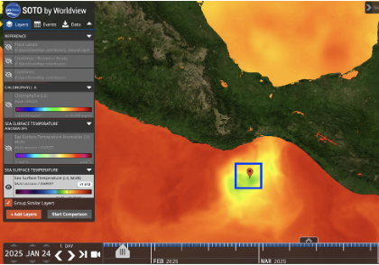
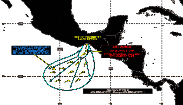
%%time

# Define region 
# Gulf of Tehuantepec, MX
lat_min = 14.
lat_max = 15.
lon_min = -96.
lon_max = -95.

lat_range = (lat_min, lat_max)
lon_range = (lon_min, lon_max)

# for datasets that use 0-360 deg lon
lon_range_360 = (lon_min+360, lon_max+360)

# Define the time slice 
start_date = '1993-01-01'
end_date = '2002-12-31'
#end_date = '1994-12-31'
time_range =(start_date, end_date)

CPU times: user 4 μs, sys: 0 ns, total: 4 μs
Wall time: 6.2 μs

Resample spatial SST and Wind Speed means to a common monthly time step and load into memory

%%time

# A concise method to subset, resample, and average the xarray data all on one line
sst_resample = sst_ds.analysed_sst.sel(lon=slice(*lon_range), lat=slice(*lat_range), time=slice(*time_range)
).mean(["lat", "lon"]).resample(time="1ME").mean().load()

wind_speed_resample = wind_ds.ws.sel(longitude=slice(*lon_range_360), latitude=slice(*lat_range), time=slice(*time_range)
).mean(["latitude", "longitude"]).resample(time="1ME").mean().load()

CPU times: user 5min 30s, sys: 35.4 s, total: 6min 6s
Wall time: 3min 35s

Resample the wind directions means to the same common monthly time step and find the favorable wind direction and speed times

%%time

# Resample u and v winds (monthly mean)
u_resample = wind_ds.uwnd.sel(
    longitude=slice(*lon_range_360),
    latitude=slice(*lat_range),
    time=slice(*time_range)
).mean(["latitude", "longitude"]).resample(time="1ME").mean().load()

v_resample = wind_ds.vwnd.sel(
    longitude=slice(*lon_range_360),
    latitude=slice(*lat_range),
    time=slice(*time_range)
).mean(["latitude", "longitude"]).resample(time="1ME").mean().load()

#  Resample wind direction
wind_dir_resample = wind_ds.wind_direction.sel(
    longitude=slice(*lon_range_360),
    latitude=slice(*lat_range),
    time=slice(*time_range)
).mean(["latitude", "longitude"]).resample(time="1ME").mean().load()

CPU times: user 23min 50s, sys: 1min 4s, total: 24min 55s
Wall time: 9min 3s

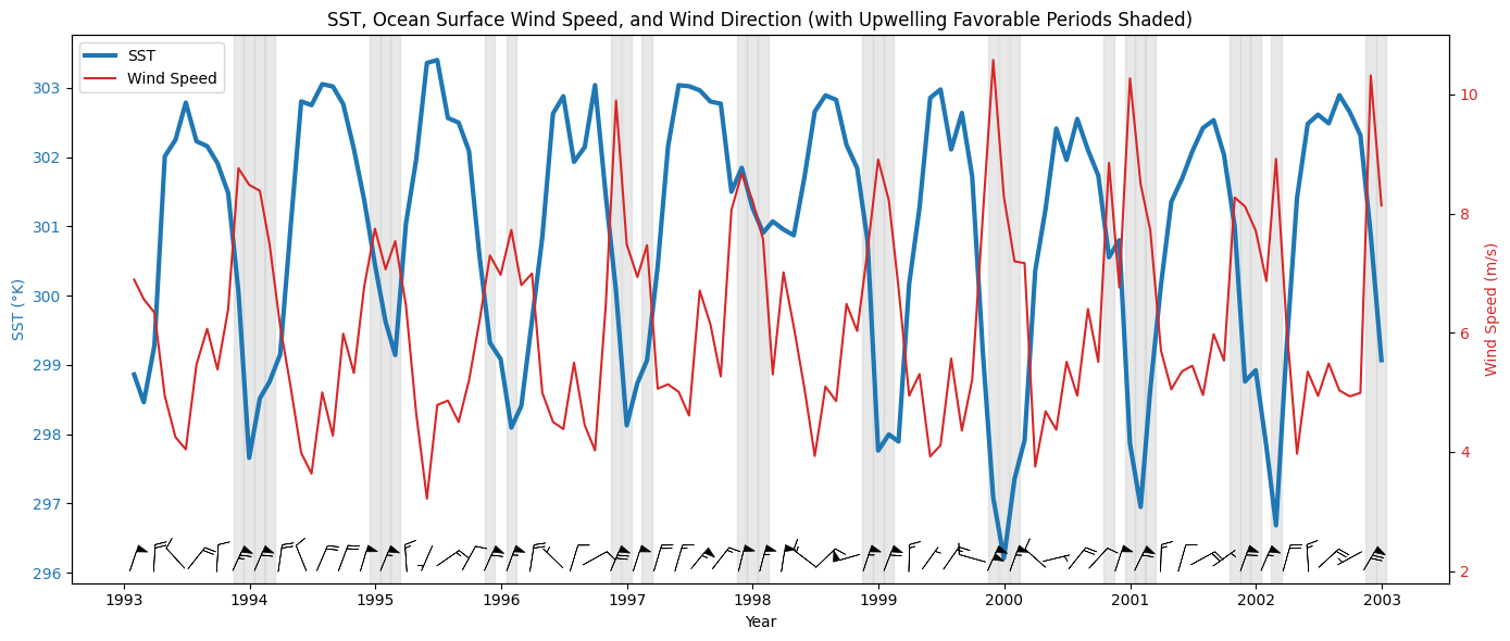
# Identify favorable wind direction times (0–120 degrees) and speeds of at least 7 m/s
favorable_mask = (wind_dir_resample >= 0 ) & (wind_dir_resample <= 120) & (wind_speed_resample >= 7)
favorable_times = wind_dir_resample.time[favorable_mask]

Check with a plot

fig, ax1 = plt.subplots(figsize=(14, 6))

# SST Plot
color = 'tab:blue'
ax1.set_xlabel('Year')
ax1.set_ylabel('SST (°K)', color=color)
ax1.plot(sst_resample['time'], sst_resample, linewidth=3, color=color, label='SST')
ax1.tick_params(axis='y', labelcolor=color)

# Wind Speed Plot
ax2 = ax1.twinx()
color = 'tab:red'
ax2.set_ylabel('Wind Speed (m/s)', color=color)
ax2.plot(wind_speed_resample['time'], wind_speed_resample, color=color, label='Wind Speed')
ax2.tick_params(axis='y', labelcolor=color)


# Add vertical shaded regions for favorable wind direction periods
for ft in favorable_times.values:
    ax1.axvspan(ft - np.timedelta64(15, 'D'), ft + np.timedelta64(15, 'D'),
                color='lightgray', alpha=0.5)

# Add wind barbs in lower panel (directional vectors)
# Normalize u and v components for visual length
barb_skip = 2  # Plot every nth point to reduce clutter if needed
barb_scale = 30  # Adjust scale for clarity

# Only plot barbs every few months
barb_time = u_resample.time.values[::barb_skip]
u_plot = u_resample.values[::barb_skip]
v_plot = v_resample.values[::barb_skip]

# Set position for barbs slightly below wind speed line
barb_y = np.full_like(u_plot, wind_speed_resample.min().item() - 1)

# Barbs on ax2 (wind axis)
ax2.barbs(barb_time, barb_y, u_plot, v_plot,
          length=6, pivot='middle', barb_increments=dict(half=1, full=2, flag=5),
          color='k', linewidth=0.5)

# Add legend
lines_1, labels_1 = ax1.get_legend_handles_labels()
lines_2, labels_2 = ax2.get_legend_handles_labels()
ax2.legend(lines_1 + lines_2, labels_1 + labels_2, loc='upper left')

plt.title("SST, Ocean Surface Wind Speed, and Wind Direction (with Upwelling Favorable Periods Shaded)")
fig.tight_layout()
plt.show()

Use parallel processing to speed the resample() approach

# Set up parallel processing

# Check how many cpu's are on this VM:
print("CPU count =", multiprocessing.cpu_count())

# Start up cluster and print some information about it:
client = Client(n_workers=32, threads_per_worker=1)
print(client.cluster)
print("View any work being done on the cluster here", client.dashboard_link)

CPU count = 32

/opt/coiled/env/lib/python3.12/site-packages/distributed/node.py:182: UserWarning: Port 8787 is already in use.
Perhaps you already have a cluster running?
Hosting the HTTP server on port 39349 instead
  warnings.warn(

LocalCluster(e9b7ad80, 'tcp://127.0.0.1:45251', workers=32, threads=32, memory=122.27 GiB)
View any work being done on the cluster here https://cluster-weliu.dask.host/jupyter/proxy/39349/status

%%time

# Execute Tasks: Convert to weekly (1W) monthly (1ME) or annual means (1YE).  
# use load() to load into memory the result

# A concise method to subset, resample, and average the xarray data all on one line
sst_resample = sst_ds.analysed_sst.sel(lon=slice(*lon_range), lat=slice(*lat_range), time=slice(*time_range)
).mean(["lat", "lon"]).resample(time="1ME").mean().load()

wind_speed_resample = wind_ds.ws.sel(longitude=slice(*lon_range_360), latitude=slice(*lat_range), time=slice(*time_range)
).mean(["latitude", "longitude"]).resample(time="1ME").mean().load()

u_resample = wind_ds.uwnd.sel(
    longitude=slice(*lon_range_360),
    latitude=slice(*lat_range),
    time=slice(*time_range)
).mean(["latitude", "longitude"]).resample(time="1ME").mean().load()

v_resample = wind_ds.vwnd.sel(
    longitude=slice(*lon_range_360),
    latitude=slice(*lat_range),
    time=slice(*time_range)
).mean(["latitude", "longitude"]).resample(time="1ME").mean().load()

wind_dir_resample = wind_ds.wind_direction.sel(
    longitude=slice(*lon_range_360),
    latitude=slice(*lat_range),
    time=slice(*time_range)
).mean(["latitude", "longitude"]).resample(time="1ME").mean().load()

# Trigger computation with parallel execution....optional
sst_data, wind_speed_data, u_data, v_data, wind_dir_data = da.compute(sst_resample, wind_speed_resample, u_resample, v_resample, wind_dir_resample)

Check with a plot

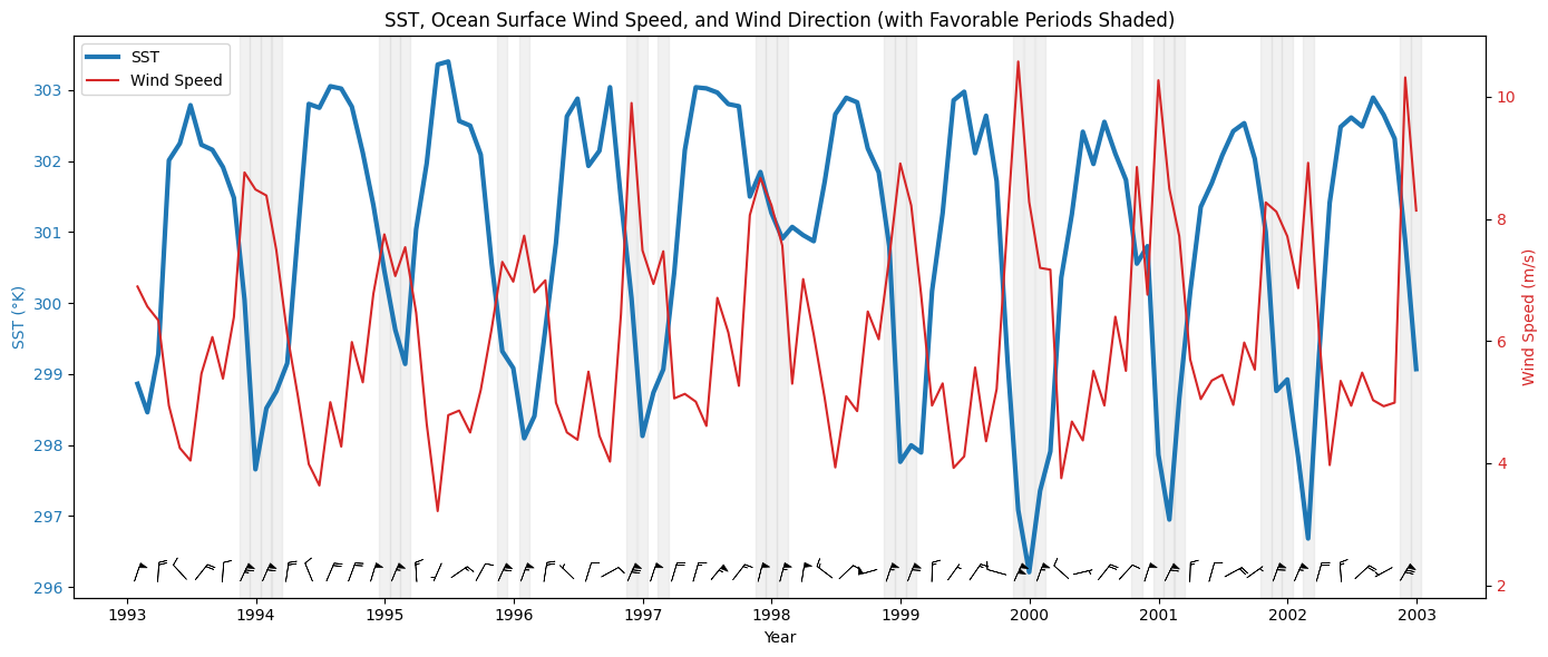
# Identify favorable wind direction times (0–120 degrees) and speeds of at least 7 m/s
favorable_mask = (wind_dir_resample >= 0 ) & (wind_dir_resample <= 120) & (wind_speed_resample >= 7)
favorable_times = wind_dir_resample.time[favorable_mask]

fig, ax1 = plt.subplots(figsize=(14, 6))

# SST Plot
color = 'tab:blue'
ax1.set_xlabel('Year')
ax1.set_ylabel('SST (°K)', color=color)
ax1.plot(sst_resample['time'], sst_resample, linewidth=3, color=color, label='SST')
ax1.tick_params(axis='y', labelcolor=color)

# Wind Speed Plot
ax2 = ax1.twinx()
color = 'tab:red'
ax2.set_ylabel('Wind Speed (m/s)', color=color)
ax2.plot(wind_speed_resample['time'], wind_speed_resample, color=color, label='Wind Speed')
ax2.tick_params(axis='y', labelcolor=color)

# Add vertical shaded regions for favorable wind direction periods
for ft in favorable_times.values:
    ax1.axvspan(ft - np.timedelta64(15, 'D'), ft + np.timedelta64(15, 'D'),
                color='lightgray', alpha=0.3)

# Add wind barbs in lower panel (directional vectors)
# Normalize u and v components for visual length
barb_skip = 2  # Plot every nth point to reduce clutter if needed
barb_scale = 30  # Adjust scale for clarity

# Only plot barbs every few months
barb_time = u_resample.time.values[::barb_skip]
u_plot = u_resample.values[::barb_skip]
v_plot = v_resample.values[::barb_skip]

# Set position for barbs slightly below wind speed line
barb_y = np.full_like(u_plot, wind_speed_resample.min().item() - 1)

# Barbs on ax2 (wind axis)
ax2.barbs(barb_time, barb_y, u_plot, v_plot,
          length=5, pivot='middle', barb_increments=dict(half=1, full=2, flag=5),
          color='k', linewidth=0.5)

# Add legend
lines_1, labels_1 = ax1.get_legend_handles_labels()
lines_2, labels_2 = ax2.get_legend_handles_labels()
ax2.legend(lines_1 + lines_2, labels_1 + labels_2, loc='upper left')

plt.title("SST, Ocean Surface Wind Speed, and Wind Direction (with Favorable Periods Shaded)")
fig.tight_layout()
plt.show()

references :

Mears, C.; Lee, T.; Ricciardulli, L.; Wang, X.; Wentz, F. Improving the Accuracy of the Cross-Calibrated Multi-Platform (CCMP) Ocean Vector Winds. Remote Sens. 2022, 14, 4230. https://doi.org/10.3390/rs14174230, Atlas, R., R. N. Hoffman, J. Ardizzone, S. M. Leidner, J. C. Jusem, D. K. Smith, D. Gombos, 2011: A cross-calibrated, multiplatform ocean surface wind velocity product for meteorological and oceanographic applications. Bull. Amer. Meteor. Soc., 92, 157-174. https://doi.org/10.1175/2010BAMS2946.1